Fragility Metrics Documentation
Fragility metrics provide a general framework for quantifying how robust or fragile statistical results are to small changes in the underlying data. The p–fr–nb framework described here is designed to apply across a wide range of study designs, including binary, continuous, and time-to-event outcomes.
This documentation covers classical fragility measures such as the Fragility Index (FI), Fragility Quotient (FQ), and Modified-arm Fragility Quotient (MFQ), as well as more general extensions including the Global Fragility Index (GFI) and GFQ. It also outlines fragility methods for ANOVA, regression models, and other settings beyond simple two-arm 2×2 tables.
The content below is synced automatically from the official
FRAGILITY_METRICS.md file in the
fragility-metrics GitHub repository
.
FRAGILITY METRICS v14.4.0
The Fragility-Robustness Framework: Unified Metrics for Statistical Evidence Quality Across Discrete and Continuous Outcome Types
Thomas F. Heston Department of Family Medicine, University of Washington, Seattle, WA, USA Department of Medical Education and Clinical Sciences, Washington State University, Spokane, WA, USA ORCID: 0000-0002-5655-2512 Version: 14.4.0
Date: September 19, 2026
Abstract
A p-value of 0.049 and a p-value of 0.0001 are both reported as 'statistically significant'—but they represent vastly different levels of evidence quality. The p–fr–nb framework fixes this. Instead of reporting p-values alone ("partial evidence"), we propose complete statistical evidence, defined as the triplet p–fr–nb: the p-value (significance), a native fragility quotient fr (classification stability), and a neutrality-boundary robustness metric nb (distance from therapeutic neutrality). Fragility (fr) is first quantified by native fragility quotients that measure the proportion of relevant data (or SE-scale shift) required to flip significance classification within a given design, with primary metrics MFQ, GFQ (gold standard for r×c and multinomial), DFQ (diagnostic benchmarks), BFQ (single-arm benchmarks), CFQ (continuous outcomes via Welch t-geometry), PFI (fixed-margin designs), ANOVA-FQ (multi-group continuous outcomes), ZFQ (the Fisher-z Fragility Quotient; correlations), OFQ (ordinal outcomes via Wilcoxon-Mann-Whitney z-statistic), SFQ (survival outcomes via Cox regression z-statistic), and WFQ (the Wald Fragility Quotient; fallback for any effect estimate reported with a Wald z-statistic or 95% CI when no design-native metric applies). fr is the native fragility quotient for the design at hand (MFQ, GFQ, CFQ, …), computed directly from the observed data; high fr indicates a stable classification, low fr indicates fragility. Native quotients are not numerically comparable across designs; a cross-design percentile scale is a deferred extension (see Part I). Robustness (nb) quantifies geometric distance from therapeutic neutrality via the Neutrality Boundary Framework (NBF), with primary metrics RQ (independent-sample binary/multinomial), MHQ (matched-pair/fixed-margin designs), DNB (diagnostic odds ratio), Proportion-NBF (single-arm benchmarks and agreement vs chance), MeCI (continuous means), DTI (correlation), ANOVAη² (multi-group), ORQ (ordinal outcomes), and SRQ (survival outcomes). All metrics use only observed counts or published summary statistics; no raw data, simulation, reconstruction, or covariate models permitted. Fragility always measures classification stability (high fr is desirable when the p-value supports the claim). Robustness interpretation is claim-dependent: high nb supports "effect exists" claims, undermines "no effect" claims. This document finalizes the integration of continuous-outcome measures (CFQ, MeCI, ANOVA-FQ, ZFQ), single-arm benchmark measures (BFQ + Proportion-NBF), and the unified fr/nb notation, providing a complete evidence-quality system applicable to nearly every standard study design with minimal assumptions. We define "complete statistical evidence" as the p–fr–nb triplet: p for significance, fr for fragility, and nb for robustness, replacing partial evidence based only on statistical significance or nonsignificance.
Keywords: statistical fragility, statistical robustness, neutrality boundary framework, fragility index, continuous fragility quotient, evidence quality metrics, p-value limitations, model-free statistics
Executive Summary
Whereas p < 0.05 establishes statistical significance, a concordant p–fr–nb triplet (low p + high fr + high nb) establishes convincing, complete statistical evidence. Traditional practice reports only the p-value for a given analysis, which we term partial evidence: it addresses compatibility with the null but not the stability of that decision or the distance from therapeutic neutrality. We define complete statistical evidence as the triplet (p, fr, nb), where p quantifies statistical significance; fr is the native fragility quotient for the design (MFQ, GFQ, CFQ, etc.), a 0–1 measure of the proportion of data or SE-shift needed to flip significance — high fr means the classification is stable, low fr means unstable; and nb is a 0–1 robustness metric measuring geometric distance from the neutrality boundary. Only when all three dimensions align (low p, high fr, high nb for "effect exists" claims) do we regard the statistical evidence as complete in the sense of being decision-ready and replication-ready. Reporting only p-values yields partial evidence, because it ignores both the stability of the conclusion (fragility) and the distance from neutrality (robustness). The p–fr–nb triplet restores these missing dimensions and constitutes complete statistical evidence for a result.
Quick Start: Your First p–fr–nb Triplet
You have a 2×2 table from a binary outcome trial: | | Events | Non-events | |---------|--------|------------| | Treatment | 13 | 87 | | Control | 25 | 75 | Calculate:
- p = 0.046 (Fisher's exact, two-sided)
- fr = MFQ = 0.01 (1 toggle / 100 in the treatment arm; changing a single treatment-arm outcome from non-event to event raises p to 0.073, losing significance)
- nb = RQ = 0.12 (|ad − bc| / (N²/4) = 1200 / 10000) Interpret: p-significant, fr-unstable, nb-intermediate → Classic unstable result: significance rests on a single outcome. Treat as low-quality evidence; replicate before use. Calculators: https://doi.org/10.5281/zenodo.17254763
The Statistical Evidence Framework
Modern evidence assessment rests on three complementary statistical dimensions plus clinical effect size: | Secret question from every skeptical reader | p alone answers | p–fr–nb triplet answers | |-------------------------------------------------------------------------------|-----------------|--------------------------------------------------------------| | Significant? | Yes | Yes (p) | | Flippable by a few outcome changes or dropouts? | ? | Yes — fr quantifies the fragility of the p-value | | Real separation from zero, or just lucky sampling noise that barely hit p<0.05? | ? | Yes — nb quantifies distance from the neutrality boundary | Only when all three dimensions align strongly (low p + high fr + high nb) do we have truly compelling, replication-ready evidence that an intervention works.
Definitions
Probability (p-value): the p-value quantifies the compatibility of the observed data with the null hypothesis (no effect). Lower p-values indicate stronger evidence against the null hypothesis. Conventional threshold: p < 0.05 for "statistically significant." Fragility (fr): the fragility summary statistic, fr, measures the stability of the significance classification. A high fr indicates stability, i.e., it takes a significant shift in outcomes to flip significance. A low fr indicates fragility, i.e., it takes only a slight change in outcomes to flip significance. Fragility quantifies the minimal perturbation to the data required to reverse the p-value decision. fr ∈ [0,1] is the native fragility quotient for the design (e.g., MFQ, GFQ, CFQ), computed directly from the observed data. fr is a perturbation-fragility metric. Part I places it within the broader taxonomy of analysis fragility and data fragility, with resampling, perturbation, and scaling as the three data-fragility forms. Robustness (nb): The robustness summary statistic, nb, measures how far the observed result sits from therapeutic neutrality (no effect), expressed as a bounded, sign-agnostic standardized effect magnitude on a 0–1 scale. nb ∈ [0,1] where high nb = far from neutrality and low nb = near neutrality. nb is a property of the point estimate: it is computed from the observed effect magnitude, not from its precision — sampling uncertainty is carried by p and by fragility, not by nb. This separation is deliberate: it is what lets the triplet distinguish a large-but-imprecise effect (high nb, unstable) from a genuinely null one (low nb), and it is what the founding metric RQ already does (RQ is scale-invariant — multiplying every cell of a 2×2 by a constant leaves it unchanged). Here "robustness" denotes distance from therapeutic neutrality — a standardized effect magnitude — and not the classical statistical sense of insensitivity to modeling assumptions or outliers. A high nb indicates the result is far from neutrality; a low nb indicates it is statistically close to neutrality (which is not, by itself, affirmative evidence that no effect exists). nb is comparable across trials within a design; native nb values are not equivalent across designs (empirically they diverge), so cross-design nb supports a common interpretive language (near/intermediate/far), not numerical equivalence. Effect size: the magnitude of the observed effect. Two magnitudes matter, and the framework now separates them cleanly. The relative, standardized magnitude — how far the effect sits from no effect on a common 0–1 scale — is captured by nb itself: SRQ reparametrizes ln(HR), DTI reparametrizes atanh(r), and the rest of the transform family behaves the same way. The absolute magnitude — mean difference in native units, absolute risk reduction, number needed to treat, months of survival gained — is not recoverable from nb, and it is the quantity the fourth element supplies. Like nb, the absolute effect size is a property of the point estimate, independent of statistical significance and sampling uncertainty. The split is therefore relative magnitude (nb, inside the triplet) versus absolute magnitude (effect size, the fourth element), not "should I believe it" versus "how much better," since the triplet already speaks to relative magnitude through nb. A large relative effect can still be a trivial absolute one: halving risk from 2% to 1% yields a healthy nb but a number needed to treat of 100. Complete evidence therefore pairs the triplet with the absolute effect size; clinical decisions require both. Partial Evidence: reporting of p-values alone or p-values with 95% CIs only constitutes "partial evidence." Complete Statistical Evidence: a result is considered to have complete statistical evidence only when all three dimensions of the p–fr–nb triplet are reported together: significance (p-value), fragility (fr), and robustness (nb). Traditional reporting of the duplet p-values with 95% confidence intervals (CI) constitutes "partial evidence." The p-value addresses only compatibility with the null hypothesis, while the 95% CI quantifies precision and effect size, but does not directly measure classification stability or normalized strength of evidence for a non-zero effect. The CI tells you the range of plausible effect sizes but not how many outcome changes would flip statistical significance (fragility); nor does it provide a standardized measure of how strong the evidence is that a real, non-zero effect exists (this is what robustness quantifies on a 0–1 scale). Complete evidence requires assessing all three dimensions to determine whether a finding is decision-ready and replication-ready. Recommended reporting thus includes complete statistical evidence (p–fr–nb) plus the non-statistical (but critical) quantity, effect size. Complete Evidence: The p–fr–nb triplet plus effect size (the quartet). Complete evidence requires both the inferential assessment (is the finding real, stable, and separated from null?) and the magnitude assessment (how large is the effect?).
The Three Statistical Dimensions
1. Statistical Significance (p)
- Question: How compatible are the data with the null?
- Scale: 0 to 1
- Interpretation: Lower p = stronger evidence against the null
2. Fragility (fr)
Native fragility quotients (fr ∈ [0,1])
- Question: What proportion of the data (or of an SE-scale shift) must change to flip the significance classification?
- Native metrics: FQ, MFQ, GFQ, CFQ, SFQ, ZFQ, OFQ, ANOVA-FQ, PFI, DFQ, BFQ
- Interpretation: Lower fr = less stable; higher fr = more stable. fr is the native quotient for the design at hand, computed directly from the observed data; the p–fr–nb triplet uses this native quotient as its fragility coordinate.
Cross-design normalization (deferred). Native quotients are not numerically comparable across designs (binary medians run lower than continuous). A percentile-normalized universal scale is a planned extension pending published reference distributions; until then, fr is interpreted within its design family.
3. Robustness (nb ∈ [0,1])
- Question: How far is the result from the neutrality boundary?
- Unified metric: nb (all NBF metrics output nb directly)
- Interpretation: Higher nb = farther from the neutrality boundary
Key Insight: Interpretation Depends on Your Claim
Claiming an effect exists (p ≤ 0.05): Prefer low p, high fr, high nb. Only when all three align strongly do we have truly compelling evidence.
Claiming no effect (p > 0.05): Prefer high p, high fr, low nb.
The measurements are universal; the interpretation is claim-dependent.
In most common trial designs, the framework provides paired metrics (both fr and nb) so stability and distance from neutrality can be evaluated together (e.g., MFQ + RQ, PFI + RQ, DFQ + DNB, CFQ + MeCI, ANOVA-FQ + ANOVAη²).
Part I: Conceptual Framework
The Three Dimensions of Evidence Quality (All 0–1)
1. Probability (p-value)
- Concept: provides the probability of the result given the null hypothesis being true
- Scale: 0 to 1
- Metric: p-value as determined by any number of statistical techniques
- Typical Interpretation: p < 0.05 = findings are significant. p ≥ 0.05 = findings are not significant.
2. Fragility (Proportion-based or Scale-based Stability)
- Concept: Quantifies the stability of a significance classification on a scale of 0 (unstable) to 1 (stable).
- Native notation: q_m ∈ [0,1] for each metric m.
- Measures: Proportion of the sample (binary/diagnostic) or proportion of an SE-scale shift (continuous) required to flip the p-value classification.
- Scale: 0 to 1 (native fragility quotients).
- Primary native metrics: FQ, MFQ, GFQ, DFQ, BFQ, PFI, CFQ, ANOVA-FQ, ZFQ, OFQ, SFQ, WFQ (generic Wald fallback).
- Secondary metrics: FI, SFI, GFI, FD (the fragility distance, with aFD, dFD), DFI, CFS, WFS (raw counts/units).
- Interpretation (native): Lower q_m = less stable; higher q_m = more stable.
Cross-Design Comparability
Native fragility quotients (MFQ, GFQ, CFQ, SFQ, ZFQ, OFQ, ANOVA-FQ, PFI, DFQ, BFQ, WFQ) provide direct physical interpretation within each study design, but their raw values have not been validated to be comparable across designs. A universal cross-design scale via percentile normalization against reference distributions is a possibility. Pending further work, fr is the native quotient, interpreted within its design family.
Taxonomy of Statistical Fragility
Statistical fragility describes the stability of the significance classification. The taxonomy identifies which component of a study is allowed to vary while that classification is assessed. It first separates analysis fragility from data fragility. Data fragility then divides into resampling fragility, perturbation fragility, and scaling fragility. These are four forms of statistical fragility, not four interchangeable estimates of one quantity.
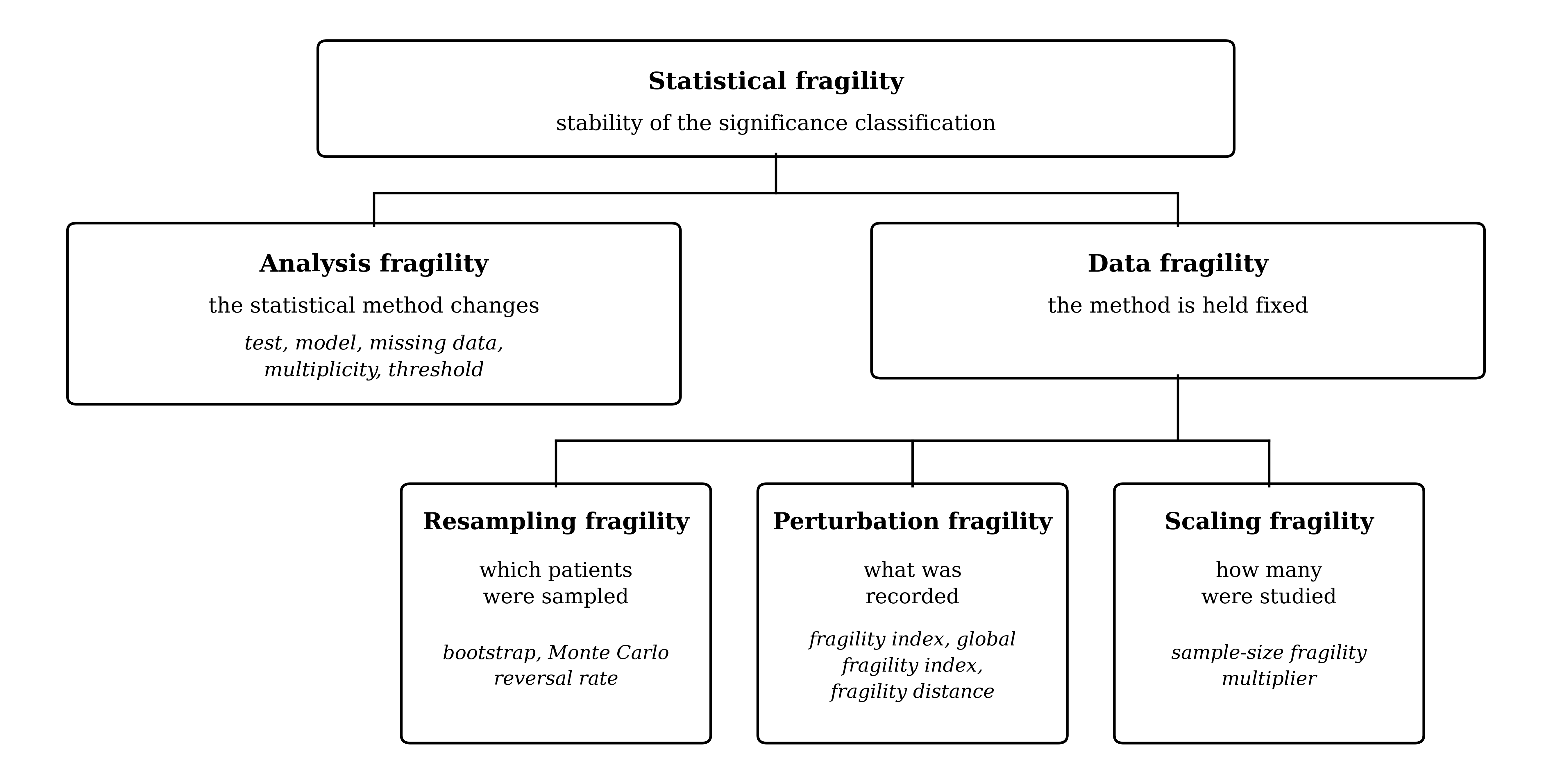
Figure 1. The four forms of statistical fragility. Analysis fragility changes the analytical rule. Data fragility holds that rule fixed and changes which patients are sampled, what is recorded, or how much data is studied.
| Branch | Form | What changes | What is held fixed | Assessment and units |
|---|---|---|---|---|
| Analysis fragility | Analysis | The analytical rule | The observed data | Classification under alternative analyses; report each rule, p-value, and classification |
| Data fragility | Resampling | Which patients are sampled | Sample size, analytical rule, and specified sampling process | Estimated probability or percentage of replicate samples that reverse classification |
| Data fragility | Perturbation | Recorded outcomes or particular patient counts | Analytical rule and the metric's stated constraints | Minimum toggles, transfers, or unit edits; matching quotient, or continuous boundary distance |
| Data fragility | Scaling | The amount of data | Observed proportions, allocation ratio, and analytical rule | Sample-size fragility multiplier (SFM), a scaling factor |
Analysis fragility. The observed data remain fixed while the analytical rule changes. Choices include the statistical test and its convention, covariate adjustment, handling of missing data, multiplicity correction, interim stopping rule, and significance threshold. Analysis fragility comes first in the logical order: each subsequent data-fragility assessment requires a fixed analytical rule. Changing the test during a perturbation search mixes analysis and perturbation fragility and prevents interpretation as a single perturbation count.
Resampling fragility (RF). This is the estimated probability that the original significance classification would reverse in another sample of the same size under a specified data-generating process. It may be estimated by bootstrap resampling or Monte Carlo simulation under a specified or fitted population model, with the analysis and threshold held fixed. It concerns hypothetical samples and depends on the resampling procedure or population model. It is recognized in the taxonomy but remains outside the operational p–fr–nb triplet because it introduces sampling assumptions beyond a direct measurement of the observed evidence. A reversal probability is not an outcome-edit count.
Number needed to reverse (NNR). NNR = 1/RF: the number of identical repeat trials expected to produce one reversal of the significance classification. It is the replication companion of the number needed to treat — no information beyond RF, a repackaging onto the scale of counted trials. Under the normal approximation, RF is a function of the p-value alone: with z = Phi^-1(1 - p/2), RF = Phi(1.96 - z) - Phi(-1.96 - z) for a significant baseline and the complement for a nonsignificant baseline, so NNR is computable from p at any sample size. Anchors: NNR = 2.0 at p = 0.05; 2.4 at p = 0.03; 3.7 at p = 0.01; 5.0 at p = 0.005; 10.9 at p = 0.001; 37 at p = 0.0001. For counted outcomes under the Fisher exact test the closed form is approximate, with deviations confined to small sparse tables. NNR, like RF, sits outside the operational p–fr–nb triplet and is claim-symmetric: for a significant baseline it counts expected repeats until a nonsignificant result, and for a nonsignificant baseline the reverse. RF was labeled RV (resampling variability) in early program output; RF and NNR are the canonical names.
Perturbation fragility. This measures the minimum change to the recorded data required to reverse significance under a fixed analytical rule and a declared move set. For binary tables, FI toggles outcomes within the specified arm; GFI transfers patients between any cells while holding N fixed; FD adds or removes one patient from one cell at a time, with N and margins free. A toggle or transfer changes two cells and costs two L1 units; one FD edit changes one cell and costs one L1 unit. Thus FD ≤ 2·GFI under the same test, not necessarily FD ≤ GFI. Particular patient removals, including loss-to-follow-up scenarios, belong here even though N changes: they do not preserve the observed proportions as scaling does.
The matching quotients retain their existing definitions: MFQ = FI / n_mod; GFQ = GFI / N; FDQ = min(1, FD / m), where m is the smallest margin of the observed table. These denominators answer different questions and do not make the quotients numerically interchangeable. Continuous measures such as CFQ express perturbation as distance in the specified test-statistic geometry rather than an integer count of patients. The fr coordinate of the p–fr–nb triplet remains a native perturbation-fragility quotient.
Scaling fragility. This measures the effect of changing sample size while holding the observed proportions constant. SFM gives the factor by which the table must grow or shrink to reverse classification. For proportional scaling of a contingency table, use Pearson chi-square without continuity correction because the scaled cells can be fractional; use that same test for the baseline and the scaled tables. A Fisher-based baseline must not be combined with a Pearson-based scaling result without reporting that change of analysis separately. SFM is a scaling-fragility measure, not a perturbation quotient or a neutrality-boundary robustness metric (see Part VII).
Interpretation and reporting. Name the form before reporting a fragility value. State the analytical rule, threshold, baseline classification, permitted change, and output units; for resampling, also state the sampling model or bootstrap procedure. A trial may be stable under one form and unstable under another without contradiction. All four assess classification stability; none by itself measures effect size, clinical importance, or freedom from bias. Changing the target to a boundary incorporating clinical importance changes the decision boundary, not which component is varied. The operational target in this document remains statistical-significance classification.
Relation to the framework. The taxonomy is broader than the triplet's fr coordinate. Analysis and resampling assessments and the secondary SFM describe other sources of classification instability; they do not replace fr or nb. Correlation with the p-value does not, by itself, establish that different forms measure the same quantity. The model-free requirement for operational framework metrics and the distinction between significance-boundary fragility and neutrality-boundary robustness remain in force.
Source: Thomas F. Heston, A Taxonomy of Statistical Fragility in Clinical Trials: Analysis, Resampling, Perturbation, and Scaling, supplied manuscript manuscript04_v4.docx. This section incorporates its conceptual taxonomy; metric formulas retain the canonical definitions given in this document.
3. Robustness (Geometric Distance)
- Concept: Quantifies the distance from therapeutic neutrality on a scale of 0 (neutral) to 1 (robust separation).
- Unified notation: nb ∈ [0,1]
- Measures: Geometric distance from the neutrality boundary (no effect).
- Scale: 0 to 1 (NBF normalized)
- Primary metrics: RQ (independent-sample binary/multinomial), MHQ (matched-pair/fixed-margin designs), DNB, Proportion-NBF, MeCI, DTI, ANOVAη² → all compute nb
-
Interpretation: Lower nb = near neutrality; higher nb = far from neutrality.
The Interpretation Layer
Measurement ≠ Interpretation Robustness (nb) has opposite implications depending on the claim being made: | Claim | High Robustness (far from neutral) | Low Robustness (near neutral) | | ------------------------------ | ---------------------------------- | ----------------------------- | | "Effect exists" (p ≤ 0.05) | Supports the claim | Undermines the claim | | "No effect" (p > 0.05) | Undermines the claim | Supports the claim | Fragility (fr) behaves differently:
- Low fr (near 0): unstable — small outcome changes flip the significance classification
- High fr (near 1): stable — the significance classification is well-supported Unlike nb, fr is claim-invariant: higher fr always strengthens confidence in the observed classification — whether significant or nonsignificant — and lower fr always weakens it. Only nb's interpretation flips with the claim.
Part II: Quick Reference Table
| Metric | Type | Scale | Primary/Secondary | Formula (core) | Purpose |
|---|---|---|---|---|---|
| FQ | Fragility | 0–1 | LEGACY | FI / N | Proportion to flip (Walsh-derived, total N) |
| MFQ | Fragility | 0–1 | PRIMARY | FI / n_mod | Proportion to flip (arm-specific) |
| GFQ | Fragility | 0–1 | PRIMARY | GFI / N | Proportion to flip (global, r×c) |
| DFQ | Fragility | 0–1 | PRIMARY | DFI / n_relevant | Proportion to flip (diagnostic) |
| BFQ | Fragility | 0–1 | PRIMARY | BFI / n_relevant (n_relevant = n) | Proportion to flip (single-arm vs benchmark) |
| CFQ | Fragility | 0–1 | PRIMARY | ||T| − t*| / (1 + ||T| − t*|) | SE-scaled distance to p = 0.05 (continuous) |
| PFI | Fragility | 0–1 | PRIMARY | 4 × |x| / N (x = fixed-margin path shift) | Independent-sample 2x2 sub-integer fragility |
| RQ | Robustness | 0–1 | PRIMARY | Σ|O − E| / [2N(m − 1)/m], m = min(r, c); for any 2×2 this equals Σ|O − E| / N = |ad − bc| / (N²/4) | Distance from independence |
| sRQ | Robustness | −1–+1 | PRIMARY | 4(ad − bc) / N² (signed RQ; |sRQ| = RQ) | Signed distance from independence |
| wsRQ | Robustness | −1–+1 | PRIMARY (meta) | Σ(sRQ_i · w_i), w_i = N_i/ΣN | Pooled signed meta-analytic robustness |
| wGFQ | Fragility | 0–1 | PRIMARY (meta) | Σ(GFQ_i · w_i), w_i = N_i/ΣN | Pooled meta-analytic fragility |
| MHQ | Robustness | 0–1 | PRIMARY (matched) | |b − c| / (b + c) or 0 if b + c = 0 | Distance from marginal homogeneity |
| DNB | Robustness | 0–1 | PRIMARY | |ln(DOR)| / (1+|ln(DOR)|) | Diagnostic distance from neutrality |
| Proportion-NBF | Robustness | 0–1 | PRIMARY | |p̂ − p₀| / (|p̂ − p₀| + √[p₀(1 − p₀)/n_relevant]) | Single-arm distance from benchmark / chance agreement |
| MeCI | Robustness | 0–1 | PRIMARY | d / (1 + d) where d = min(|μ₁−c|, |μ₂−c|) / √(s₁²+s₂²), c = (s₁μ₂+s₂μ₁)/(s₁+s₂) | Continuous distance from neutrality |
| DTI | Robustness | 0–1 | PRIMARY | |atanh(r)| / (1 + |atanh(r)|) | Correlation distance from independence |
| ZFQ | Fragility | 0–1 | PRIMARY | |Z − 1.96| / (1 + |Z − 1.96|) where Z = |atanh(r)|√(n−3), n > 3 | Correlation classification stability (Fisher-z) |
| OFQ | Fragility | 0–1 | PRIMARY | ||z_WMW| − 1.96| / (1 + ||z_WMW| − 1.96|) | SE-scaled distance to p = 0.05 (ordinal) |
| ORQ | Robustness | 0–1 | PRIMARY | |ln(gOR)| / (1 + |ln(gOR)|) | Distance from neutrality (ordinal) |
| ANOVA-FQ | Fragility | 0–1 | PRIMARY (k≥2) | |√F − √F| / (1 + |√F − √F|) | Stability of F-classification |
| ANOVAη² | Robustness | 0–1 | PRIMARY | df_b·F / (df_b·F + df_w) | Distance from equality of means |
| FI | Count | 0–N | Secondary | Toggle count (single-arm) | Raw fragility count (binary) |
| SFI | Count | 0–N | Secondary | Toggle count (standardized) | Label-invariant count |
| GFI | Count | 0–N | Secondary | Move count (global) | Path-independent count |
| FD | Count (edit distance) | 0–∞ | Secondary | min # unit edits (add or remove one patient in any cell; N free) to cross p = 0.05 (Fisher) | Fragility distance: unconstrained L1 edit distance to the significance boundary |
| FDQ | Fragility | 0–1 | Secondary | min(1, FD / m), m = smallest margin of the observed table (n_A, n_B, a+c, b+d); flagged margin-limited when FD > m | Fragility distance as a fraction of the scarce margin (not on the GFQ scale) |
| aFD | Count (edit distance) | 0–∞ | Secondary | FD search restricted to additions only (N grows) | Addition-only edit distance; upper bound on FD |
| dFD | Count (edit distance) | 0–N | Secondary | FD search restricted to deletions only (N shrinks) | Deletion-only edit distance; upper bound on FD |
| DFI | Count | 0–N | Secondary | Toggle count vs benchmark | Diagnostic count |
| NDI | Count (robustness) | 0–N/4 | Secondary | round(N·RQ/4) = round(|ad − bc|/N), clamped to reachability | Coupled fixed-margin moves to neutrality (RR = 1) |
| CFS | Distance | 0–∞ | Secondary | ||T| − t*| | SE-unit distance to p = 0.05 (continuous) |
| SFM | Scaling | > 1 | Secondary | Factor k > 1 to flip (×k flips nonsignificant → significant; ÷k flips significant → nonsignificant) | Sample size fragility multiplier |
| UFI | Unit | >0 | LEGACY | N/(n₁n₂) or 1/max(n₁, n₂) or 1/N | Step-size definitions (fixed-margin unit size) |
| SFQ | Fragility | 0–1 | PRIMARY | ||z_HR| − 1.96| / (1 + ||z_HR| − 1.96|) | SE-scaled distance to p = 0.05 (survival) |
| SRQ | Robustness | 0–1 | PRIMARY | |ln(HR)| / (1 + |ln(HR)|) | Distance from neutrality (survival) |
| WFQ | Fragility | 0–1 | PRIMARY (fallback) | ||z| − 1.96| / (1 + ||z| − 1.96|), z = θ̂ / SE (SE from 95% CI) | SE-scaled distance to p = 0.05 (generic Wald; only when no design-native metric applies) |
| WFS | Distance | 0–∞ | Secondary | ||z| − 1.96| | SE-unit distance to p = 0.05 (generic Wald) |
| t* is the critical value from the t-distribution. | |||||
| F* is the critical F value at α = 0.05 for the reported df. | |||||
| m = min(r, c). The denominator 2N(m − 1)/m is the maximum of Σ | O − E | , attained under perfect association; for 2×2 it equals N, so 2×2 values are unchanged. |
Part III: PRIMARY FRAGILITY METRICS
Core Concept
Naming rule (Walsh FI). The 2014 single-arm toggle index is referred to as the Walsh FI (or, for the bidirectional minimum, the Heston FI). The adjective "classic" is banned as a name for it throughout canon, manuscripts, and code comments: it asserts stature, not definition. Refer to metrics by originator or by mechanism (single-arm toggle, transfer, edit).
Fragility quotients measure the proportion of the sample (binary/diagnostic) or the proportion of SE-scale movement (continuous) required to flip statistical significance. All primary native fragility quotients range 0–1 (MFQ, GFQ, CFQ, SFQ, etc.). fr is the native fragility quotient for the design at hand, computed directly from the observed data. Cross-design percentile normalization is a deferred extension (see Part I), not part of the operational framework.
3.1 FQ — Fragility Quotient
Application: Legacy metric for any binary outcome 2×2 table (independent samples) using total N denominator. Definition: Proportion of the total sample that must toggle to flip significance Formula: FQ = FI/N Range: 0 to 1 Interpretation: fr = FQ (the native quotient). For example, FQ = 0.02 means 2% of sample outcomes must change to flip statistical significance. Advantages: use for historical comparison with studies that used FQ Base metric: FI (Heston fragility index) NBF pair: RQ Note: FQ is a legacy metric and is not recommended as the primary fr metric for 2-arm binary outcome studies. GFQ is preferred (path-independent and label-invariant); when large N makes GFI computation intractable, MFQ is the fallback, which is allocation-fair (denominating against the arm actually modified) and label-resistant.
3.2 MFQ — Modified-arm Fragility Quotient ⭐
Application: Fallback for independent-sample 2×2 binary outcome trials (any allocation ratio) when large sample size (≈5000+) makes GFI computation intractable, or when compatibility with the Walsh FI count is required. Definition: Proportion of the arm that was actually modified in the Walsh fragility index procedure required to flip statistical significance. Formula: MFQ = FI / n_mod, where n_mod = sample size of the arm subjected to toggling in the standard FI calculation (i.e., the arm with fewer events; if tied, the smaller arm). Range: 0 to 1 Interpretation: fr = MFQ. Example: MFQ = 0.05 means 5% of patients in the arm that was toggled would need to switch outcome to flip significance. Advantages: allocation-resistant: minimizes the distortion caused by unequal study allocation; the MFQ is label-resistant but not label independent like the GFQ is. Base metric: Heston FI NBF pair: RQ Note: For 2×2 binary outcome tables, GFQ is the recommended default (§3.3); use MFQ when GFI is computationally intractable at large N, or when comparability with the universally recognized FI count is needed. MFQ remains allocation-fair by denominating against the arm that actually needs to change. When MFQ is used, pair it as MFQ + RQ.
3.3 GFQ — Global Fragility Quotient ⭐
Application: Recommended default and gold standard for any r×c contingency table or multinomial outcomes (independent samples), including 2×2 binary outcome trials. Definition: Proportion of sample involved in minimal cell moves Formula: GFQ = GFI/N Range: 0 to 1 Interpretation: For GFQ, fr = GFQ (e.g., GFQ = 0.03 means 3% of the sample must be reallocated to flip statistical significance). Advantages: Path-independent, applies to any r×c table Base metric: GFI (global fragility index) NBF pair: RQ Note: Considered the gold standard for binary and multinomial fragility assessment because of its path-independence and label-invariance, and it is the recommended default for 2×2 binary outcome tables. For large sample sizes (≈5000+), computing GFI becomes computationally intractable, and MFQ becomes the practical fallback for two-arm binary outcome studies (§3.2). The GFQ complements RQ, which measures robustness (distance from independence). Both should be reported together — GFQ + RQ is the standard pair for binary and multinomial outcomes. Both the GFI and the GFQ show label-invariance.
3.4 DFQ — Diagnostic Fragility Quotient ⭐
Application: Diagnostic metrics from full 2×2 table (TP, FN, FP, TN) with ground truth. Definition: Proportion of the relevant subset of observations that must toggle to change the diagnostic classification (below vs not below benchmark) using a one-sided exact binomial test against p₀, paired with DNB. Formula: DFQ = DFI / n_relevant, where n_relevant depends on the metric:
- Sensitivity: n_relevant = TP + FN (disease+)
- Specificity: n_relevant = TN + FP (disease−)
- PPV: n_relevant = TP + FP (test+)
- NPV: n_relevant = TN + FN (test−)
- ACCURACY (agreement with truth): n_relevant = TP + FN + FP + TN = N
Range: 0 to 1
Interpretation: For DFQ, fr = DFQ (e.g., DFQ = 0.06 means 6% of the relevant cases must change to flip the benchmark classification).
Advantages: Correctly targets the subset of observations that determine each diagnostic metric, and uses a one-sided exact test appropriate for benchmark comparisons.
Base metric: DFI (diagnostic fragility index)
NBF pair: DNB
Note: Uses a one-sided exact binomial test against the investigator-specified benchmark p₀:
H₀: p = p₀ vs H₁: p < p₀ (for “below benchmark” diagnostic standards); the direction may be reversed (H₁: p > p₀) when the claim is framed as meeting or exceeding the benchmark, matching the direction convention of BFQ (§3.5).
For agreement against chance, p₀ = 0.5 is standard. For PPV/NPV/ACCURACY, data should be normalized to 50% disease prevalence (see §3.4.1). DFQ assesses fragility (stability of the benchmark classification) for diagnostic metrics derived from a full 2×2 table with ground truth. It complements DNB, which measures robustness (distance of the diagnostic odds ratio from neutrality). Both should be reported together for diagnostic accuracy studies. For single-arm benchmark analyses based only on (k, n, p₀), use BFQ + Proportion-NBF instead of DFQ + DNB.
3.4.1 Prevalence Normalization for PPV/NPV/ACCURACY (Standard Procedure)
Rationale: We cannot compare a test's PPV/NPV/ACCURACY across studies unless the underlying prevalence is normalized. Since clinical testing is most helpful when diagnostic uncertainty is high (pretest ≈ 50%), prevalence is set to 50%. Procedure:
- Identify minority class: min(n_disease+, n_disease−)
- Scale the majority class to match the minority, preserving its internal ratio:
- If scaling disease−: maintain FP:TN
- If scaling disease+: maintain TP:FN
- Round conservatively: TP/TN down, FP/FN up
- Calculate DFI on the normalized table
- DFQ = DFI / n_relevant_normalized
3.5 BFQ — Benchmark Fragility Quotient ⭐
Application: Single-arm benchmark tests and agreement vs benchmark when only (k, n, p₀) are available. Typical use cases: a) Single-arm response rate vs a benchmark proportion p₀ b) Single-rater agreement vs chance (p₀ = 0.5) or another target benchmark when the full TP/FN/FP/TN table is not available Definition: Proportion of observations in a single-arm proportion that must toggle (success ↔ failure) to change the benchmark classification under a one-sided exact binomial test. Formula: BFQ = BFI / n_relevant, where:
- n_relevant = n (denominator of the observed proportion)
- BFI = minimal number of success/failure toggles that flips the one-sided exact binomial test classification at the benchmark proportion p₀ Test: One-sided exact binomial test vs benchmark p₀
- H₀: p = p₀
- H₁: p > p₀ (for “above benchmark” claims; direction may be reversed if the benchmark is framed as a maximum allowable rate). Range: 0 to 1 Interpretation: fr = BFQ (e.g., BFQ = 0.08 means 8% of the observations in the single-arm proportion must change to flip the benchmark decision). Advantages:
- Establishes the fragility of a single-arm test, giving a success rate vs the benchmark.
- Applies when only (k, n, p₀) are available (no full diagnostic 2×2 table).
- Mirrors the DFQ logic but in a single-arm setting.
- Uses the same exact binomial test that defines the underlying benchmark decision. Base metric: BFI (Benchmark Fragility Index) = minimal number of success/failure toggles required to change the benchmark classification under the specified one-sided exact binomial test. NBF pair: Proportion-NBF Note: Use BFQ when the analysis is “proportion/agreement vs a benchmark” based only on (k, n, p₀). For full diagnostic accuracy studies with TP/FN/FP/TN and a diagnostic odds ratio, use DFQ + DNB instead. Common applications:
- Single-arm response rates vs historical control
- Agreement vs chance (p₀ = 0.5) when no ground truth available
- Any proportion vs pre-specified benchmark
3.6 PFI — Percent Fragility Index⭐
Application: independent-sample binary 2×2 trials (continuous analog of FI/SFI/UFI for sub-integer fragility resolution). Definition: Proportion of one balanced cell's expected count that must be reallocated along a fixed-margin perturbation path to flip the Pearson chi-square significance classification in an independent-sample 2×2 design. Formula: PFI = |x| / (N/4) = 4|x| / N, where x is the smallest margin-preserving change in the four cells, applied along the path (a+x, b−x, c−x, d+x), that flips the two-sided Pearson chi-square decision across the α = 0.05 boundary (sign ignored), and N/4 is the expected count per cell in a perfectly balanced 2×2 under independence. For reporting, PFI is conventionally multiplied by 100 and expressed as a percent (e.g., PFI = 0.02 is reported as 2%). Range: 0 to 1 (native quotient; reported as 0% to 100%). Bounded by construction for significance flips: along the fixed-margin path the cross-product difference is linear, Δ(x) = (ad − bc) + xN, so the independence point (Δ = 0) sits at |x| = |ad − bc| / N ≤ N/4 (since |ad − bc| ≤ N²/4). The two-sided chi-square boundary is crossed at or before independence, hence x_flip ≤ N/4 and PFI = 4|x_flip|/N ≤ 1. Boundary-limited cases (below) are capped at 1.0. Significance test: Pearson chi-square, without Yates correction. Fisher's exact does not admit fractional counts, so it cannot resolve sub-integer flips; Yates correction is omitted because it is designed for integer counts, adds conservative bias, and disrupts the smoothness of χ² that continuous perturbation requires. Interpretation: fr = PFI. Lower PFI indicates greater fragility. PFI = 0.02 (2%) means a 2% proportional shift in outcome distribution, relative to the balanced-cell expected count, would reverse significance. Provisional guidance (subject to empirical testing): PFI < 0.05 (5%) is concerning for fragility; PFI > 0.10 (10%) suggests relatively stable findings. Advantages: a) detects sub-integer fragility that integer metrics (FI, SFI) cannot represent; b) label-agnostic — no determination of minority arm or event coding required; c) margin-preserving, so perturbations reflect proportional redistribution within the observed trial structure; d) continuous scale aligns naturally with the framework's other continuous fragility metrics (CFQ, SFQ, ZFQ, OFQ) and supports smooth percentile normalization to fr. Base metric: x (minimal margin-preserving cell perturbation along the fixed-margin path) NBF pair: RQ Note: The fixed-margin path is a sensitivity construct, not a claim that the trial had fixed margins by design. It holds row sums (arm sizes) and column sums (total events) constant so that any admissible change is a coupled diagonal exchange, isolating sensitivity to proportional redistribution. The continuous (chi-square) criterion is required for sub-integer resolution; PFI is a descriptive evidence-quality metric, not an inferential test, so the perturbation geometry and the significance criterion need not share a single likelihood. For strictly matched-pair or crossover designs in which both margins are fixed by the design itself, McNemar-based fragility (with MHQ robustness) is the design-coherent choice; PFI as defined here targets the independent-sample case.
- Boundary-limited cases: When the feasible shift range along the fixed-margin path is exhausted before the chi-square p-value can cross α = 0.05 (e.g., the table is already at maximal directional imbalance), no admissible perturbation flips significance. In these cases, PFI returns the maximum feasible proportion along the path, capped at 1.0 (100%), and is flagged "boundary-limited," indicating maximal stability of the current classification under the fixed-margin constraint.
- PFI values are not numerically comparable to GFQ or MFQ because they assess fragility under different perturbation models and significance criteria.
- Sub-integer realizability (Type C, 2026-07-11): the perturbed intermediate table (a+x, b−x, c−x, d+x) with non-integer x is not itself a realizable contingency table, and PFI does not claim it is. Here x is a distance to the significance boundary measured in proportional-reallocation units, not a count of changed patients — in the same sense that a p-value is a continuous functional of a discrete table with no single realizable table sitting exactly 'at' p = 0.0493. The concrete gain over the integer fragility index is resolution within ties: many trials share FI = 1 or FI = 2 yet differ in how close they truly sit to α = 0.05, and PFI orders them. This is precisely why PFI is reported as a descriptive evidence-quality metric rather than an inferential test — it quantifies boundary proximity on a continuous scale, and its usefulness does not depend on the intermediate table being realizable.
- PFI-M = McNemar-path fragility = the McNemar-test variant of PFI for matched-pair designs; identical path construction, McNemar χ² in place of Pearson χ². Note that along this path b and c change by the same amount, so the McNemar numerator (b − c)² is invariant; significance flips only through the change in the discordant-pair total (b + c − 2x). PFI-M therefore probes a narrower perturbation space than PFI.
Distance-to-Critical-Value Family (§3.7–3.12)
Sections §3.7–3.12 are one construct — the bounded distance from the test statistic to its α = 0.05 critical value, fr = δ/(1 + δ) with δ = |stat − crit| — instantiated per design: continuous (CFQ), multi-group (ANOVA-FQ), correlation (ZFQ), ordinal (OFQ), survival (SFQ), and a generic Wald fallback for designs without a native metric (WFQ). The umbrella is conceptual; the per-design instances below are what you compute.
3.7 CFQ — Continuous Fragility Quotient ⭐
Application: trials comparing two continuous outcomes where m₁, m₂, s₁, s₂, n₁, n₂ are all known. Definition: Proportion of an SE-scaled shift in the estimated mean difference required to flip statistical significance in a two-sample continuous comparison (Welch t-test). Formula: Let m₁, m₂ = observed group means s₁, s₂ = observed standard deviations n₁, n₂ = group sample sizes. v₁ = s₁²/n₁ (variance of mean 1), v₂ = s₂²/n₂ (variance of mean 2), SE_diff = √(v₁ + v₂) (this is the Continuous Fragility Unit, CFU), θ̂ = m₁ − m₂ (observed mean difference), T = θ̂ / SE_diff (observed Welch t-statistic), df = (v₁ + v₂)² / (v₁²/(n₁−1) + v₂²/(n₂−1)), (Welch–Satterthwaite degrees of freedom), t = t₀.₉₇₅,df (two-sided critical value at α = 0.05). Then: Continuous Fragility Score (distance in SE units to the p = 0.05 boundary): CFS = | |T| − t |. Continuous Fragility Quotient: CFQ = CFS / (1 + CFS). Range: 0 to 1. Interpretation: fr = CFQ. For example, CFQ = 0.12 means the observed t-statistic lies relatively close to the p = 0.05 boundary on the CFQ scale; smaller values indicate a less stable significance classification, larger values a more stable one. Advantages: Works directly from reported summary statistics (m₁, m₂, s₁, s₂, n₁, n₂). No raw data required. No simulated data or distributional reconstruction. Correctly respects Welch's variance structure and degrees of freedom. Provides a continuous-outcome analogue of MFQ/GFQ. Base metric: CFS = continuous fragility score (SE-unit distance between |T| and t*). NBF pair: MeCI Note: CFQ assesses fragility (stability of significance). It complements MeCI, which assesses robustness (distance from neutrality). Both should be reported for continuous outcomes. CI-only implementation note: When only a 95% CI for the mean difference is available, T and SE are reconstructed using a large-sample z-based approximation (t ≈ 1.96). Under this approximation, p and CFS/CFQ values are asymptotic. MeCI cannot be computed from a mean-difference CI alone because the crossover-point formula requires separate group means and SDs; in CI-only scenarios, report CFQ alone or reconstruct group-level summary statistics where possible. Note on Paired/Matched Data: For crossover trials, pre-post measurements, or matched pairs, the CFQ formula applies directly using the paired t-statistic:
- T_paired = mean_diff / (s_diff / √n)
- Degrees of freedom = n − 1 (paired)
- CFS = | |T_paired| − t* |
- CFQ = CFS / (1 + CFS) For MeCI in paired designs, compute the crossover point between the two measurement conditions (e.g., pre/post means and SDs, or crossover arms 1/2) using the standard crossover-point formula c = (s₁·μ₂ + s₂·μ₁)/(s₁+s₂), then MeCI = d/(1+d) where d = min(|μ₁−c|, |μ₂−c|) / √(s₁²+s₂²). MeCI in paired designs uses the group-level summary statistics of the two conditions, not the paired-differences summary.
3.8 ANOVA-FQ — ANOVA Fragility Quotient ⭐
Application: One-way ANOVA with k ≥ 2 independent groups (continuous outcome, equal or unequal variances assumed by the reported F-test). Definition: Bounded (0–1) distance in √F space from the α = 0.05 classification boundary. At k = 2, √F space coincides exactly with the SE-scaled t space of CFQ; for k > 2 it serves as the analogous distance scale. Formula: ANOVA-FS = |√F − √F| ANOVA-FQ = ANOVA-FS / (1 + ANOVA-FS) where F is the critical F value at α = 0.05 for the reported (df_b, df_w). Range: 0 to 1 Interpretation: fr = ANOVA-FQ (higher = more stable classification) Advantages:
- Model-free (uses only reported F and df)
- Path-independent (√F geometry is unique)
- Reduces exactly to CFQ when k = 2 and the F-test and t-test share the same variance assumption: a pooled-variance F reduces to the pooled-variance Student-t form of CFS (F = t² → √F = |t|, and √F = t); a Welch F reduces to the Welch-based CFQ as defined in §3.7. When variance assumptions differ (pooled-variance F vs Welch CFQ under heteroscedasticity), the correspondence is approximate, not exact.
- Completes the p–fr–nb triplet for one-way ANOVA designs Base metric: ANOVA-FS (raw fragility score in √F units) NBF pair: ANOVAη² (official robustness metric, unchanged) Note: Supersedes previous v9.6 statement that “no model-free fragility exists for k>2”. The √F transformation provides a canonical, assumption-free distance metric that satisfies all framework requirements. Effective v10.0, one-way ANOVA has a complete p–fr–nb triplet. Reference: Heston TF. Extending the Fragility Quotient to Multi-Group ANOVA via √F Geometry. (in preparation, 2025)
3.9 ZFQ — Fisher-z Fragility Quotient (Correlation) ⭐
Application: Pearson or Spearman correlation reported as (r, n), with n > 3 and |r| < 1. Definition: Symmetric fragility metric measuring distance from the α = 0.05 classification boundary in Fisher-z space. Formula: Let z_r = atanh(r), Z = |z_r|√(n−3), Z_crit = 1.96 D = |Z − Z_crit| ZFQ = D / (1 + D) For Spearman correlations, the Fisher-z variance is inflated; use the Fieller/Bonett–Wright adjustment Z = |atanh(r_s)| · √((n−3)/1.06) in place of the Pearson form. Domain: Requires n > 3 (√(n−3) undefined otherwise) and |r| < 1 (atanh diverges at ±1). Range: 0 to 1 Interpretation: fr = ZFQ. Higher values indicate more stable classification (significant or non-significant). Advantages: Sample-size dependent, symmetric around decision boundary, structurally identical to CFQ/ANOVA-FQ Base metric: D (distance in Fisher-z test statistic units) NBF pair: DTI Note: Completes the p–fr–nb triplet for correlation analyses. ZFQ measures classification stability; DTI measures robustness (distance from independence). Both required for complete correlation evidence assessment.
3.10 OFQ — Ordinal Fragility Quotient ⭐
Application: Ordinal outcomes analyzed via Wilcoxon-Mann-Whitney test, proportional odds models, or ordinal logistic regression (e.g., modified Rankin Scale, NIHSS, pain scales, functional status scores). Definition: Proportion of SE-scaled shift in the ordinal test z-statistic required to flip statistical significance for ordinal outcomes. Formula: Let gOR = generalized odds ratio (common odds ratio from proportional odds model), with 95% CI [CI_lower, CI_upper], where gOR, CI_lower, and CI_upper are all > 0. Calculate:
- ln(gOR) = natural log of the generalized odds ratio
- SE_log_gOR ≈ [ln(CI_upper) − ln(CI_lower)] / (2 × 1.96) (standard error reconstructed from the confidence interval)
- z ≈ ln(gOR) / SE_log_gOR (Wald z-statistic for ln(gOR); under the proportional odds assumption this approximates the Wilcoxon-Mann-Whitney z-statistic, denoted z_WMW) Then: OFQ = | |z_WMW| − 1.96 | / (1 + | |z_WMW| − 1.96 |) Range: 0 to 1 Interpretation: fr = OFQ. Example: OFQ = 0.33 means the z-statistic is moderately far from the p = 0.05 boundary on the OFQ scale; higher values indicate more stable significance classification (significant or non-significant). Advantages: Works directly from reported gOR and 95% CI (standard reporting for ordinal outcomes). No raw data, ranks, or distributional assumptions beyond proportional odds required. Extends the fragility framework to ordinal shift analysis. Base metric: | |z_WMW| − 1.96 | (raw distance in z-statistic units to the two-sided significance boundary) NBF pair: ORQ Note: OFQ assesses fragility (stability of significance classification) for ordinal outcomes. It complements ORQ, which measures robustness (distance from neutrality). Both should be reported together for ordinal outcome studies. Structurally identical to CFQ (continuous), ANOVA-FQ (multi-group), and ZFQ (correlation). Because z is reconstructed from the CI via a Wald approximation, OFQ values are asymptotic; when the exact WMW z-statistic is reported directly, use it in place of the CI reconstruction.
3.11 SFQ — Survival Fragility Quotient ⭐
Application: Time-to-event outcomes analyzed via Cox regression (e.g., overall survival, progression-free survival, time to heart failure hospitalization). Definition: Proportion of SE-scaled shift in the Cox regression z-statistic required to flip statistical significance for survival outcomes. Formula: Let HR = hazard ratio from Cox regression, with 95% CI [CI_lower, CI_upper]. Calculate:
- ln(HR) = natural log of the hazard ratio
- SE_ln_HR ≈ [ln(CI_upper) - ln(CI_lower)] / (2 × 1.96) (standard error from confidence interval)
- z_HR = ln(HR) / SE_ln_HR (Cox z-statistic) Then: SFQ = | |z_HR| − 1.96 | / (1 + | |z_HR| − 1.96 |)
Range: 0 to 1 Interpretation: fr = SFQ. Example: SFQ = 0.15 means the z-statistic is relatively close to the p = 0.05 boundary on the SFQ scale; higher values indicate more stable significance classification. Advantages: Works directly from reported HR and 95% CI (standard reporting for survival outcomes). No raw survival data, Kaplan-Meier curves, or censoring information required. Extends the fragility framework to time-to-event analysis. Base metric: | |z_HR| − 1.96 | (raw distance in z-statistic units to significance boundary) NBF pair: SRQ Note: SFQ assesses fragility (stability of significance classification) for survival outcomes. It complements SRQ, which measures robustness (distance from neutrality). Both should be reported together for time-to-event studies. Structurally identical to CFQ (continuous), ANOVA-FQ (multi-group), ZFQ (correlation), and OFQ (ordinal).
3.12 WFQ — Wald Fragility Quotient ⭐
Application: Fallback metric for any effect estimate reported with a Wald-type z-statistic, or with a 95% confidence interval from which one can be reconstructed, when no design-native metric in this document applies — e.g., regression coefficients (linear, logistic, Poisson, survey-weighted), prevalence or trend slopes, risk differences, and adjusted mean changes. Precedence rule: WFQ is never used where a design-native metric is computable. A Cox hazard ratio takes SFQ; a generalized odds ratio takes OFQ; a correlation takes ZFQ; two-group continuous summary statistics take CFQ; a multi-group F-test takes ANOVA-FQ; a contingency table takes GFQ (or MFQ at large N). WFQ covers the remainder. Definition: Bounded distance, in standard-error units, between the observed Wald z-statistic and the two-sided α = 0.05 critical value. Formula: Let θ̂ = reported effect estimate with 95% CI [CI_lower, CI_upper] on the same scale (for ratio measures — which the precedence rule routes to their native metrics — the estimate and CI are log-transformed first). Calculate:
- SE ≈ (CI_upper − CI_lower) / (2 × 1.96) (standard error reconstructed from the confidence interval; when the analysis reports z, or t with large df, directly, use it and skip the reconstruction)
- z = θ̂ / SE (Wald z-statistic) Then: WFS = | |z| − 1.96 | (Wald Fragility Score: raw SE-unit distance to the significance boundary) WFQ = WFS / (1 + WFS) Range: 0 to 1 Interpretation: fr = WFQ. Defined for both significant and nonsignificant baselines (classification stability in either direction). Example: WFQ = 0.48 means the z-statistic sits 0.92 SE units from the p = 0.05 boundary (the map is invertible: WFS = WFQ/(1 − WFQ)); higher values indicate a more stable significance classification. Advantages: Works directly from the estimate + 95% CI pair, the most common summary format in the literature. No raw data, no model refitting. Structurally identical to CFQ, ANOVA-FQ, ZFQ, OFQ, and SFQ, extending the fragility framework to designs the named metrics do not reach. Base metric: WFS NBF pair: none for non-ratio estimates. Ratio estimates never reach WFQ (the precedence rule routes them to native metrics with native NBF pairs). For non-ratio coefficients — slopes, differences, adjusted changes — no nb metric is currently defined: the triplet is incomplete for this design, and results are reported as p–fr plus the absolute effect size with an explicit statement that nb is unavailable. Do not improvise an nb transform; defining one is future work. Note: z reconstructed from a CI is a Wald approximation, so WFQ values are asymptotic, matching the CI-only conventions of CFQ, OFQ, and SFQ. The critical value is fixed at 1.96 (normal approximation); when the source analysis used a t-reference with small degrees of freedom, use that t-critical value in place of 1.96 and state so. Because WFQ is a deterministic monotone function of |z| alone, within this design it is a re-expression of the reported test onto the boundary-distance scale — it adds interpretive resolution near the α boundary, not information beyond the reported statistic; design-native metrics that read table geometry (GFQ) remain preferred wherever computable, per the precedence rule. Case matters in the acronym family: uppercase-W WFQ/WFS are the generic Wald metrics; lowercase-w metrics (wGFQ, wsRQ, wFDQ) are the weighted meta-analytic pooled forms, and the two groups are unrelated.
Part IV: Primary Robustness Metrics
Core Concept: Neutrality Boundary Framework (NBF)
NBF metrics quantify geometric distance from neutrality—where treatment equals control (e.g. RR=1, Δ=0, r=0, DOR=1).
General NBF Formula: NBF = |T − T₀| / (|T − T₀| + S), where T = statistic, T₀ = neutral value, and S = a fixed, sample-independent scale parameter (commonly S = 1, giving the x/(1+x) bounding map). S is not a standard error: nb depends on the effect magnitude, not its precision.
Universal property: all NBF metrics → [0,1].
Interpretation: 0 = at neutrality, 1 = maximally separated.
Distance-from-neutrality transform family. DTI, ORQ, SRQ, and DNB share one construct — a bounded, sign-agnostic distance from neutrality of the form |g(θ)|/(1 + |g(θ)|), where g is a variance-stabilizing transform of the effect estimate θ (atanh for correlation r; ln for the ratio metrics gOR, HR, DOR). One idea, instantiated per design; each keeps its own θ, and each is computed from the effect estimate alone, not its precision.
The NNT analogy. NBF is to effect sizes what the number needed to treat (NNT) is to the absolute risk reduction: no new information, a repackaging onto the scale where decisions are made. NNT is algebraically nothing more than 1/ARR, yet it became indispensable because it moved the same quantity onto the scale where clinical judgment operates. NBF makes the identical move for distance from neutrality. Each metric is a monotone transform of a familiar effect estimate — RQ is a normalized cross-product distance related to the phi coefficient; SRQ, ORQ, and DNB are bounded log-ratios; DTI is a bounded Fisher z — and the contribution is the common bounded scale and the claim-dependent reading, not new mathematics. The comparison limit travels with the analogy: nb supports numerical comparison within a design family; across designs it supplies a common interpretive language (near / intermediate / far), not equivalent numbers.
4.1 RQ — Risk Quotient ⭐
Application: Independent-sample binary or multinomial outcome tables (2×2 or r×c) assessing separation from independence (treatment vs control or multi-arm studies).
Definition: NBF-based robustness metric measuring geometric distance from independence in binary or multinomial outcome tables.
Formula (general): RQ = Σ|O − E| / [2N(m − 1)/m] for any r×c table, where O are observed counts, E are expected counts under independence, m = min(r, c), and the denominator 2N(m − 1)/m is the maximum attainable value of Σ|O − E| (attained under perfect association). This normalization guarantees RQ ∈ [0, 1] for every r×c table.
Special-case shortcut (for any 2×2): since m = 2 makes the denominator equal N, RQ = Σ|O − E| / N = |ad − bc| / (N²/4) for any 2×2 table.
Range: 0 to 1.
Interpretation: nb = RQ. For example, nb = 0.20 means the data sit at an intermediate separation from independence.
Neutrality: Independence of variables (e.g. ad = bc for 2×2)
Pairs with: FQ, MFQ, GFQ, PFI
Count counterpart: NDI (Part V) — the integer count of coupled fixed-margin moves to neutrality. For any 2×2 table, NDI = round(N·RQ/4) (clamped to reachability). NDI and RQ quantify the same underlying cross-product distance from neutrality in different units: NDI expresses that distance as an integer number of coupled fixed-margin moves, whereas RQ expresses it as a normalized 0–1 geometric distance. NDI:RQ therefore forms an Index:Quotient pairing by structural analogy to GFI:GFQ, but not by direct division: RQ is not NDI/N.
Note: Standard robustness measure for independent-sample binary and multinomial outcomes.
4.1.1 sRQ — Signed Risk Quotient ⭐
Application: Independent-sample 2×2 outcome tables where the direction of separation from independence (which arm is favored), not only its magnitude, must be retained — required for signed meta-analytic pooling (wsRQ). Definition: The canonical RQ with the absolute value removed, so the metric carries both distance from neutrality and direction. Formula: sRQ = 4(ad − bc) / N² Range: −1 to +1 (|sRQ| = RQ). Direction convention: For a 2×2 table with rows = arms (a, b = events, non-events of row 1; c, d = events, non-events of row 2) and the first row taken as the experimental/treatment arm, the sign of (ad − bc) reflects table orientation and must be declared per analysis. In the Zuin et al. PE-thrombolysis reanalysis convention used in canon, negative sRQ favors the experimental/treatment arm (fibrinolysis); positive sRQ favors the control/harm direction. State the orientation explicitly whenever sRQ is reported. Neutrality: Independence (ad = bc → sRQ = 0). Pairs with: MFQ, GFQ (fragility); aggregates to wsRQ (meta-analytic). Note: sRQ is a robustness metric — it measures signed distance from therapeutic neutrality, never classification stability. |sRQ| recovers the unsigned canonical RQ of §4.1. Direction is a property of the table orientation, not of the metric; the convention must be fixed before pooling.
4.2 DNB — Diagnostic Neutrality Boundary ⭐
Application: Diagnostic accuracy studies with full 2×2 tables (TP, FN, FP, TN) and ground truth, including sensitivity, specificity, PPV, NPV, and accuracy (after prevalence normalization when needed).
Definition: NBF-based robustness metric measuring the diagnostic odds ratio's (DOR) distance from neutrality.
Formula: DNB = |ln(DOR)| / (1 + |ln(DOR)|)
where:
- DOR = (TP × TN) / (FP × FN)
Range: 0 to 1.
Interpretation: For DNB, nb = DNB. For example, nb = 0.35 means the diagnostic odds ratio is clearly separated from no-discrimination.
Neutrality: DOR = 1 (test no better than chance).
Pairs with: DFQ
Note: DNB uses the uncertainty-free form |ln(DOR)|/(1 + |ln(DOR)|), placing it in the distance-from-neutrality transform family alongside DTI, ORQ, and SRQ (Part XI). The prior form |ln(DOR)|/(|ln(DOR)| + SE) was a monotone transform of the Wald z-statistic and duplicated the significance axis; the current form is the pure standardized effect magnitude, with precision carried by p and fr. When any cell is zero, ln(DOR) is undefined; apply a 0.5 continuity correction to all four cells before computing DNB. Primary robustness measure for diagnostic tests using a full 2×2 table. Apply after prevalence normalization for PPV/NPV and accuracy where appropriate (see §3.4.1). For single-arm benchmark analyses based only on (k, n, p₀), use Proportion-NBF instead of DNB.
4.3 MeCI — Meaningful Change Index ⭐
Application: Two-group independent continuous outcome studies (e.g., trials reporting group means and standard deviations for each arm; sample sizes are not required for MeCI but are needed for the paired CFQ calculation).
Definition: NBF-based robustness metric measuring distributional distinguishability for continuous outcomes, based on the equal-standardized-distance point of the two sample distributions — the point equidistant from the two group means in standard-deviation units, which coincides with the density crossover point of the two distributions only when s₁ = s₂. MeCI is p-value independent and sample-size independent.
Formula: Let μ₁, μ₂ be the observed group means and s₁, s₂ their standard deviations.
- Calculate the equal-standardized-distance point c (the density crossover point only when s₁ = s₂): - c = (s₁·μ₂ + s₂·μ₁) / (s₁ + s₂), equivalently the c solving (c − μ₁)/s₁ = (μ₂ − c)/s₂ Calculate the raw distance: - d = min(|μ₁ − c|, |μ₂ − c|) / √(s₁² + s₂²)
- Then apply the NBF bounding map for family consistency: MeCI = d / (1 + d)
- Range: 0 to 1.
Interpretation: For MeCI, nb = MeCI. Low MeCI values indicate near-equivalence between groups (high population overlap, little separation); high MeCI values indicate far separation (minimal overlap, clear distinguishability).
Neutrality: μ₁ = μ₂ (both means coincide with c; d = 0, MeCI = 0).
Pairs with: CFQ
Assumption: Crossover-point calculation assumes approximately normal group distributions. For heavily skewed or multimodal distributions, interpret with caution.
Note: Primary robustness metric for continuous outcomes. MeCI captures population-level distributional separation independent of α thresholds and sample size, complementing CFQ which measures fragility of the corresponding significance classification. The underlying distance quantity d follows the definition in Heston (2025); the canonical NBF form applies the x/(1+x) bounding map for consistency with the rest of the NBF family (DNB, DTI, ORQ). CI-only implementation note: MeCI cannot be computed from a published mean-difference CI alone, as the crossover-point formula requires separate group means and SDs. In CI-only scenarios, report CFQ alone or reconstruct group-level summary statistics where possible.
4.4 DTI — Distance to Independence ⭐
Application: Correlation/association studies where the primary result is a correlation coefficient (e.g., Pearson or Spearman r).
Definition: NBF-based robustness metric for correlations.
Formula: DTI = |atanh(r)| / (1 + |atanh(r)|)
Range: 0 to 1.
Interpretation: For DTI, nb = DTI. For example, nb = 0.25 means the correlation is clearly separated from zero.
Neutrality: r = 0
Pairs with: ZFQ
Note: Primary robustness measure for correlation studies; member of the distance-from-neutrality transform family (Part XI).
4.5 ANOVAη² ⭐
Application: Multi-group continuous outcome comparisons analysed with one-way ANOVA or equivalent F-tests.
Definition: NBF-compatible robustness metric for multi-group comparisons.
Formula: η² = df_b·F / (df_b·F + df_w)
Range: 0 to 1.
Interpretation: For ANOVAη², nb = η². For example, nb = 0.30 means substantial between-group variation relative to within-group variation.
Neutrality: All group means equal (F = 0).
Pairs with: ANOVA-FQ
Note: Equivalent to the traditional eta-squared effect size; already NBF-compatible. Now paired with ANOVA-FQ to provide complete p–fr–nb triplet for one-way ANOVA designs.
4.6 Proportion-NBF (Single-Arm Neutrality Boundary Metric) ⭐
Application: Single-arm proportion vs benchmark analyses (e.g., single-arm response rates or agreement vs benchmark) when only k, n_relevant, and p₀ are available.
Definition: Proportion-NBF measures geometric distance between an observed single-arm proportion and a benchmark proportion p₀. It is the NBF counterpart to BFQ when only k, n_relevant, and p₀ are available.
Formula:
- Let k = number of successes, n_relevant = total number of trials, p̂ = observed_proportion = k / n_relevant, p₀ = benchmark proportion used in the one-sided exact binomial test, and S = √[ p₀ × (1 − p₀) ] (fixed, sample-independent scale; provisional — see changelog).
- Then: Proportion-NBF = |p̂ − p₀| / (|p̂ − p₀| + S).
Range: 0 to 1.
Interpretation: Identical to all NBF metrics. Values near 0 indicate data lying on the neutrality boundary. Values above 0.50 reflect far separation from neutrality.
Neutrality: p̂ = p₀.
Pairs with: BFQ
Note: This metric is the geometric robustness partner to BFQ for single-proportion benchmark tests and generalizes the Agreement-NBF structure to arbitrary p₀. The special case p₀ = 0.5 corresponds to agreement vs chance (previously referred to as “Agreement-NBF”). Used for single-arm response rates compared with a benchmark p₀. Inputs: k (successes), n_relevant (denominator), p₀ (benchmark). Common applications: - Pairs with BFQ for single-arm response rates
- Agreement studies (p₀ = 0.5 for chance agreement)
- Any single-proportion benchmark comparison
4.7 MHQ — Marginal Homogeneity Quotient ⭐
Application: Matched-pair or fixed-margin 2×2 designs (e.g., crossover trials, pre–post paired binary outcomes, or any setting where McNemar’s test is appropriate).
Definition: NBF-style robustness metric for marginal homogeneity; proportion of discordant pairs that would need to switch direction to reach b = c.
Formula: MHQ = |b − c| / (b + c) if b + c > 0 else 0
Range: 0 to 1
Interpretation: nb = MHQ. Example: nb = 0.20 means 20% of discordant pairs must switch direction to reach b = c (neutrality).
Advantages: Matches the McNemar null exactly, and is intuitive for matched/paired designs.
Neutrality: b = c (marginal homogeneity)
Pairs with: McNemar-path fragility (matched-pair designs) = PFI-M (the McNemar-test variant of PFI for matched-pair designs; identical path construction, McNemar χ² in place of Pearson χ²)
Note: Used as the nb metric in fixed-margin/matched-pair modules, paired with McNemar-path fragility so that p, fr, and nb all reference marginal homogeneity. For independent-sample designs, PFI (fragility) and RQ (distance from independence) are the defaults.
4.8 ORQ — Ordinal Robustness Quotient ⭐
Application: Ordinal outcomes analyzed via Wilcoxon-Mann-Whitney test, proportional odds models, or ordinal logistic regression (e.g., modified Rankin Scale, NIHSS, pain scales). Definition: NBF-based robustness metric measuring geometric distance from neutrality (gOR = 1) for ordinal outcomes. Formula: Let gOR = generalized odds ratio (common odds ratio from proportional odds model). Then: ORQ = |ln(gOR)| / (1 + |ln(gOR)|) Range: 0 to 1 Interpretation: nb = ORQ. Example: nb = 0.23 means the ordinal outcome shows intermediate separation from neutrality; nb = 0.50+ indicates a far shift toward better outcomes. Neutrality: gOR = 1 (no ordinal shift between groups) Pairs with: OFQ Note: Primary robustness metric for ordinal outcomes. Uses natural log transformation (consistent with DNB for diagnostic odds ratios). Works from published gOR alone—no confidence interval needed for ORQ calculation (though CI is needed for OFQ). Member of the distance-from-neutrality transform family (Part XI).
4.9 SRQ — Survival Robustness Quotient ⭐
Application: Time-to-event outcomes analyzed via Cox regression (e.g., overall survival, disease-free survival, cardiovascular mortality). Definition: NBF-based robustness metric measuring geometric distance from neutrality (HR = 1) for survival outcomes. Formula: Let HR = hazard ratio from Cox regression. Then: SRQ = |ln(HR)| / (1 + |ln(HR)|) Range: 0 to 1 Interpretation: nb = SRQ. Example: nb = 0.18 means the hazard ratio shows intermediate separation from neutrality; nb = 0.50+ indicates a large reduction (or increase) in hazard. Neutrality: HR = 1 (equal hazard rates between groups; no treatment effect) Pairs with: SFQ Note: Primary robustness metric for survival outcomes. Uses natural log transformation (consistent with DNB for diagnostic odds ratios and ORQ for ordinal outcomes). Works from published HR alone—no confidence interval needed for SRQ calculation (though CI is needed for SFQ). Member of the distance-from-neutrality transform family (Part XI).
Part V: Secondary Metrics (Raw Counts & Units)
Raw Fragility Counts (Input to Quotients)
WalshFI — Walsh Fragility Index
Definition: Number of outcome toggles within one arm required to flip statistical significance from significant to nonsignificant. Only defined for baseline statistically significant 2×2 contingency tables. Defined procedurally, not as a minimum over a search space: the index is whatever count the prescribed iterative procedure yields. Toggle rule: Convert non-events to events, one at a time, in the arm with fewer events (recalculating p after each toggle) until p ≥ 0.05; not defined what to do if the event counts are tied. Test: Two-sided Fisher's exact, recalculated at each step regardless of the significance test the original trial reported. Output: Integer count → WalshFQ = WalshFI / N, WalshMFQ = WalshFI / n_mod. Note: Original metric from Walsh et al. (2014). The original empirical study applied it to RCTs with 1:1 allocation ratios; the index definition itself does not require equal allocation.
FI — Heston Fragility Index
Definition: Minimum number of outcome toggles within one arm required to flip the statistical significance classification in either direction (significant→nonsignificant or nonsignificant→significant), using a two-sided Fisher's exact test. Defined for both significant and nonsignificant baseline 2×2 contingency tables. Defined as a true minimum over the allowed toggles, not a procedural count. Toggle rule: Toggle outcomes (event ↔ non-event) in the arm with fewer events; if tied, toggle the smaller arm. Test: Two-sided Fisher's exact. Output: Integer count → FQ = FI / N, MFQ = FI / n_mod. Note: Heston modification of Walsh et al. (2014): bidirectional, defined for nonsignificant baselines, defined as a minimum, with an explicit tie rule.
LinFI - Lin Fragility Index (R Package)
Definition: Minimum total number of within-arm outcome toggles, distributed across either or both arms, required to flip the significance classification using a two-sided Fisher's exact test. Formally: min(|f₀| + |f₁|), where f₀ and f₁ are the net event-count changes in each arm.
Toggle rule: Toggle outcomes (event ↔ non-event) within an arm, preserving both arm sizes; bidirectional; either or both arms may be modified in the same solution.
Test: Two-sided Fisher's exact (package default; chi-squared and OR/RR/RD-based p-values are settable options).
Output: Integer count → LinFQ = LinFI / N; MFQ does not apply since there is no single modified arm.
Note: Generalizes the Walsh et al. (2014) metric as implemented by the fragility R package (Lin & Chu, 2022, frag.study): unlike Walsh FI, it is bidirectional (also defined for nonsignificant baselines, flipping toward significance) and is not restricted to a single pre-specified arm.
GFI — Global Fragility Index
Definition: Minimum number of cell-to-cell reallocations required to flip the statistical significance classification in an r×c contingency table, using the same significance test throughout the GFI search. Toggle rule: Any admissible cell movement; algorithm finds the minimal global path. Test: For 2×2 tables, GFI always uses the two-sided Fisher's exact test — the same test used by FI, MFI, and SFI — regardless of expected cell counts and regardless of the significance test the original trial reported. This guarantees test-coherence across the fragility metrics and preserves the structural invariant GFI ≤ MFI ≤ FI (every within-arm toggle is a unit reallocation, so the global minimum can never exceed the constrained minima when all three are scored by the same test). For r×c tables larger than 2×2, use the Fisher–Freeman–Halton exact test when computationally feasible; Pearson's chi-square is an acceptable asymptotic substitute when exact computation is intractable and expected counts are adequate (no expected cell count <1 and at least 80% of expected cell counts ≥5). The selected test remains fixed throughout the search and is not changed as cell counts are reallocated. As a sensitivity analysis only, GFI may additionally be computed under the test the original analysis prespecified; such values must be labeled with the test used and must not be mixed with Fisher-based FI/MFI/SFI values in fragility comparisons, because metrics scored under different tests are not mutually comparable and can violate the GFI ≤ MFI ≤ FI ordering by ±1 or more. Unit: Global Fragility Unit (GFU) = 1/N. Output: Integer count → GFQ = GFI / N. Note: Gold standard for binary and multinomial tables: path-independent, label-invariant, and domain-complete (defined for every table except the small-N floor, where no arrangement of N subjects can reach significance at the chosen α). GFI measures the minimum global perturbation required to reverse the classification produced by the significance test; therefore, the significance criterion must remain test-coherent across the baseline, all candidate tables, and the companion metrics (FI, MFI, SFI) it is reported alongside. For 2×2 tables the criterion is fixed at two-sided Fisher's exact; for larger r×c tables the exact test (Fisher–Freeman–Halton) is preferred, with Pearson's chi-square as the asymptotic fallback for adequately populated tables where exact computation is intractable. Exact-test GFI may be more computationally demanding than chi-square GFI. Because Fisher and chi-square p-values differ near the α boundary, GFI values computed under different tests typically differ by ±1 reallocation and must not be compared directly.
cGFI — Continuous Global Fragility Index
Definition: Minimum total continuous cell movement — measured as L1 distance / 2, i.e., the number of "subjects' worth" of mass reallocated — required to flip the statistical significance classification, in either direction, holding total N fixed and all cells ≥ 0. Cells are treated as continuous quantities, so fractional reallocations are admissible. Move rule: Any cell-to-cell reallocation, in continuous amounts. Computed exactly along all 18 canonical rays (12 single-pair moves, 6 diagonal exchanges) by closed-form polynomial root-finding on the chi-square boundary, then refined by constrained optimization (SLSQP) to capture off-ray minima. Test: Two-sided Pearson chi-square (continuous criterion, no Yates correction). Fisher's exact test is not applicable: it does not allow fractional counts, for the same reason as PFI (§3.6). Unit: Continuous; sub-integer resolution (same interpretive basis as the GFU, but no longer restricted to integer multiples of 1/N in quotient form). Output: Non-negative real number → cGFQ = cGFI / N. Undefined (NaN) only at the small-N floor, where no arrangement of N subjects can reach significance at the chosen α. Note: Continuous relaxation of the GFI. For tables scored by chi-square, cGFI ≤ GFI, since every integer reallocation path is also a continuous one; the gap between them measures how much of the integer index is quantization. Like PFI, cGFI resolves fragility differences among tables that share the same integer GFI (many tables have GFI = 1 yet sit at very different distances from the significance boundary), and like PFI it is a descriptive evidence-quality metric, not an inferential test: the intermediate fractional table need not be realizable. cGFI differs from PFI in move space — PFI is restricted to the single fixed-margin diagonal path, while cGFI minimizes over all continuous reallocation paths, so cGFI ≤ (N/4)·PFI on the common path and is the tighter boundary-distance measure.
Fragility Distance Family — FD, aFD, dFD (and FDQ)
This family is distinct from the reallocation metrics (GFI/GFQ, cGFI: N fixed, patients moved between cells) and from the toggle metrics (FI, MFI, SFI, UFI: N fixed, one or both margins fixed, outcomes switched within an arm). Fragility distance metrics let the table grow or shrink: the perturbation unit is one patient added to, or removed from, any cell.
Terminology convention — index vs distance. An index is a constrained path length: the minimum number of moves (toggles or transfers) to cross the significance boundary under a stated constraint set, where each move touches two cells at once (one down, one up) and therefore costs two L1 units. Each constraint set spawns its own index — FI, WalshFI, MFI, SFI (toggles, within-arm, N fixed), GFI (transfers, any cells, N fixed), UFI (coupled fixed-margin moves). A distance is the unconstrained L1 (Manhattan) minimum over the full space of 2×2 tables with nonnegative integer cells and free N, measured in patients (one unit edit = one patient added or removed). Because the space admits exactly one unconstrained minimum, there is exactly one fragility distance, FD; the indices are its family of constrained upper bounds (each in its own unit). FD does not distinguish additions from deletions: FD = 2 may be realized by one addition plus one deletion in different cells, which is equivalent to a transfer. aFD and dFD are the direction-constrained subcategories of FD, not separate constructs.
FD — Fragility Distance
(Formerly nGFI, the Neutral Global Fragility Index, v13.4.0–13.5.0; renamed v13.6.0. Prior changelog entries and the reference implementation filename retain the old name as historical record.)
Definition: The minimum number of unit edits — add one patient to any cell, or remove one patient from any cell — that moves the observed 2×2 table across p = 0.05 under the two-sided Fisher's exact test. N is free; row totals and column totals are free. FD is the L1 (Manhattan) edit distance from the observed table to the nearest table on the other side of the significance boundary. Defined for both significant and nonsignificant baselines (classification stability in either direction).
Edit rule: Any single-cell ±1 edit. A cell-to-cell reallocation (one deletion plus one addition) costs 2 edits, so a GFI path of length g is an FD path of length 2g.
Test: Two-sided Fisher's exact, fixed throughout the search.
Output: Integer count → FDQ = min(1, FD / m), where m is the smallest margin of the observed table, m = min(n_A, n_B, a + c, b + d), computed before any edit. FDQ is the fraction of the trial's scarce resource — the rarer outcome or the smaller arm, whichever binds — that must be added or removed to change the significance classification. The denominator is a property of the observed table, not of the witness path, so FDQ inherits FD's path-independence and needs no tie rule. Bound: for a significant baseline FD ≤ m always holds (deleting the entire smallest margin yields a degenerate table with p = 1, at cost m), so FDQ ∈ (0, 1] exactly. For a nonsignificant baseline the crossing typically adds into the scarce margin, which the margin does not bound; FD may then exceed m and FDQ is capped at 1.0 and flagged "margin-limited". The cap is a margin phenomenon, not a sample-size phenomenon: in the exhaustive N ≤ 60 enumeration (628,055 nondegenerate tables) it occurs only when m ≤ 8 (82% of nonsignificant tables at m = 1, 0.3% at m = 8) and never when m ≥ 9; in the 164-trial reference corpus 2 tables (1.2%) are capped, both nonsignificant with m = 2. Always report the raw FD and the witness table beside FDQ. Scale note: FDQ is not on the GFQ scale — GFQ remains GFI / N (fraction of the sample reallocated) because that sentence is the one readers compare with FQ and MFQ; FDQ answers a different question (fraction of the binding resource edited), and the two are not numerically interchangeable. N-denominated quotients (FQ, MFQ, GFQ, and the former FD / N) understate the perturbation in rare-event trials, where most of N could not have contributed to the flip; FDQ is the correction. (FDQ was defined as FD / N in v13.4.0–13.7.0; redefined v13.8.0.)
Mechanism: The edit path that attains FD is reported alongside the count as additions, deletions, or mixed. For significant tables the nearest crossing is usually reached by additions (diluting the effect); for nonsignificant tables usually by deletions; mixed paths occur. For nonsignificant baselines the nearest significant table may lie across neutrality (the effect direction reverses on the way to significance), so the search must cover both directions of effect, not only the observed one.
Relation to the p–fr–nb framework: FD is an fr-type (significance-boundary) metric. It says nothing about nb (distance from neutrality); RQ is kept separate and reported alongside it.
Interpretive claim (Heston): The author's position is that FD is the primary measure of perturbation fragility for a 2×2 table — the true minimum — because it removes the artificial constraints imposed by the index metrics — fixed N (GFI, FI, MFI, SFI), fixed margins (UFI), and single-arm toggling (FI, MFI, SFI). Every other integer fragility count is the same question asked under an added constraint, and each therefore bounds FD from above (see ordering below). This is stated as the author's interpretive position, not as an empirical finding.
Computation: Directed search over the four useful unit moves (for a significant table, the four edits that pull the arm rates together; for a nonsignificant table, the four that push them apart, with both direction sets searched where the crossing may lie beyond neutrality). Exact over all 1- and 2-move mixes (bisection on the edit count, then a full scan of splits); grid-bounded over 3- and 4-move mixes (coarse simplex grid, yielding an upper bound); the GFI witness (2·GFI edits) is included as a candidate. The result is exhaustively certified by enumerating every table in the signed L1 ball below the answer whenever that enumeration is feasible (row budget ≤ 30 million rows); otherwise it is reported as exact over ≤ 2-move mixes and an upper bound overall. Reference implementation: fragility_metrics_nGFI.py r5 (22-AUG-2026).
aFD — Addition-only Fragility Distance (formerly aGFI)
Definition: The same search as FD restricted to additions only: the minimum number of patients that must be added (one per edit, to any cell; no removals) to cross p = 0.05 under Fisher's exact test. N grows by aFD. Output: Integer count (may be undefined/unbounded where no finite number of additions along the admissible moves crosses the boundary; report as such). Note: aFD is the constrained upper bound on FD for the addition mechanism. For significant tables aFD and FD frequently coincide (dilution is usually the nearest crossing). Lay interpretation: aFD = k means that if the trial had enrolled just k more patients (with particular outcomes, in particular arms), the significance classification could have changed.
dFD — Deletion-only Fragility Distance (formerly dGFI)
Definition: The same search as FD restricted to deletions only: the minimum number of patients that must be removed (one per edit, from any cell; no additions) to cross p = 0.05 under Fisher's exact test. N shrinks by dFD; cells cannot go below zero. Output: Integer count, bounded by N (undefined when no deletion path crosses the boundary, e.g. the small-N floor on the significant side). Note: dFD is the constrained upper bound on FD for the deletion mechanism. For nonsignificant tables dFD and FD frequently coincide. Lay interpretation: dFD = k means that if the trial had lost just k particular patients (e.g., to follow-up), the significance classification could have changed.
Ordering within the family (always holds)
FD ≤ aFD, FD ≤ dFD, FD ≤ 2·GFI.
FD is the envelope (lower bound) of the family. aFD, dFD, and 2·GFI are upper bounds under their respective constraints (additions only, deletions only, reallocation only with N fixed). GFI is the reallocation-only member: one reallocation = one deletion plus one addition = 2 edits, which is why it enters the ordering as 2·GFI rather than GFI.
NDI — Neutrality Distance Index
Definition: The NDI is the minimum number of paired within row, fixed-margin toggles required to bring a 2×2 table to the point closest to a relative risk of 1 (the neutrality boundary where no effect is seen; the null hypothesis). Because integer toggles rarely will result in exact neutrality (RR=1; ad = bc), the NDI is the toggle count to bring the table closest to the minimum of |ad − bc|. It is defined for every 2×2 table. Toggle rule: Only within-row transfers are allowed. The toggles are coupled anti-parallel moves keeping both row and column marginal totals fixed. For example: a forward toggle {a−1, b+1, c+1, d−1} or reverse toggle {a+1, b−1, c−1, d+1} is allowed with the target being the minimum number of these paired toggles to achive the point closest to a RR=1. Only paired moves are allowed, e.g. a→b is always paired with d→c; and b→a is always paired with c→d. Cross-arm toggles are not allowed (e.g. a→c or b→d). Note: whichever toggle direction reaches the neutrality boundry in the fewest moves is allowable. Feinstein (1990) and Walter (1991) both used fixed-margins (the UFI) because Fisher's exact test conditions on both margins; margin preserving moves make the pertubation of the contingency table commensurable, and neutrality (ad = bc) is itself a within-margin statement. Formula: Each coupled move changes the cross-product difference by exactly ∓N with both margins and N held fixed — (a−1)(d−1) − (b+1)(c+1) = (ad − bc) − N — so reachable cross-product differences are spaced N apart and NDI = round(|ad − bc| / N) = round(N·RQ/4), clamped to the reachability window. Exact neutrality is attainable only when N divides (ad − bc). Reachability: The coupled move is bounded to x ∈ [−min(a, d), +min(b, c)]. Extreme or lopsided margins yield a narrow window, and NDI then reflects how little the table can move within Fisher's conditioning set. Test dependence: None. NDI depends only on ad − bc, a function of the observed cell counts; it invokes no significance test. This distinguishes it from the fragility counts (FI, GFI), whose target is a p-value threshold. NDI is a robustness metric expressed as an integer count. Domain: Always defined. Unlike the fixed-margin UFI — undefined when no reachable table flips significance — NDI's target is a minimization that always has a solution. NDI = 0 is a valid result: the observed table is already as close to neutrality as the fixed-margin moves permit. Unit: One coupled move = 1 unit, matching the published UFI. One coupled move relocates two patients (one per arm), so the fixed-margin indices (UFI, NDI) are on a per-coupled-move unit whereas single-transfer indices (GFI) are on a per-patient unit. The difference is by design, because the move-sets differ. Output: Integer count, range 0 to N/4 (since |ad − bc| ≤ N²/4). NDI is the count-based robustness metric; RQ (§4.1) is its normalized decimal partner, so NDI:RQ parallels the GFI:GFQ Index:Quotient pairing. Note: NDI = round(N·RQ/4) is an exact algebraic identity, not an empirical approximation — it follows from RQ = |ad − bc|/(N²/4) and the ∓N step size. The only departures from exactness are integer rounding (coarse near neutrality, where the lattice spacing N is large relative to a small |ad − bc|) and clamping at extreme margins where the reachability window binds. RQ is therefore not NDI/N. Note: Robustness counterpart to the fixed-margin unit fragility index (UFI, Part VII): UFI counts coupled fixed-margin moves to the significance boundary (p = 0.05); NDI counts the same coupled moves to the neutrality boundary (RR = 1). Together they instantiate both boundaries of the framework with one move-set. NDI is model-free (computed from the 2×2 summary counts alone, no distributional assumptions) and measures distance-to-neutrality in patient units, which p-values do not measure; it is not a transformation of p.
DFI — Diagnostic Fragility Index
Definition: Minimum number of "success" toggles required to switch the diagnostic benchmark classification between "below benchmark" and "not below benchmark" (one-sided exact binomial).
Toggle rule:
• Sensitivity: TP ↔ FN
• Specificity: TN ↔ FP
• PPV: TP ↔ FP
• NPV: TN ↔ FN
• Accuracy: any TP/TN/FP/FN toggle changing success proportion
Test: One-sided exact binomial test vs benchmark p₀.
Output: Integer count → DFQ = DFI / n_relevant.
Note: Underlying count for DFQ; always paired with DNB for diagnostic accuracy studies.
BFI — Benchmark Fragility Index
Definition: Minimum number of success/failure toggles in a single-arm binomial experiment required to switch the benchmark classification between "meets benchmark" and "does not meet benchmark" under a one-sided exact binomial test.
Toggle rule: Toggle individual outcomes (success ↔ failure) in the single arm until the one-sided exact binomial decision crosses the α = 0.05 boundary at the specified benchmark p₀.
Test: One-sided exact binomial test vs benchmark p₀.
Output: Integer count → BFQ = BFI / n_relevant (with n_relevant = n).
Note: Underlying count for BFQ in single-arm proportion vs benchmark analyses; used together with Proportion-NBF as the robustness partner.
CFS — Continuous Fragility Score
Definition: SE-unit distance between the observed Welch t-statistic and the α = 0.05 significance boundary.
Formula: CFS = ||T| – t*|.
Output: Raw distance → CFQ = CFS / (1 + CFS).
Note: Continuous analogue of FI/SFI/GFI.
WFS — Wald Fragility Score
Definition: SE-unit distance between the observed (or CI-reconstructed) Wald z-statistic and the two-sided α = 0.05 significance boundary, for generic estimates covered by WFQ (§3.12).
Formula: WFS = ||z| − 1.96|.
Output: Raw distance → WFQ = WFS / (1 + WFS).
Note: Generic-Wald analogue of CFS; asymptotic when z is reconstructed from a 95% CI.
Part VI: Continuous Fragility Units
CFU — Continuous Fragility Unit
Welch model (two independent continuous groups):
v₁ = s₁² / n₁
v₂ = s₂² / n₂
CFU = SE_diff = √(v₁ + v₂)
Purpose: One SE-shift in the estimated mean difference under Welch.
CFS — Continuous Fragility Score
CFS = ||T| − t*|
Defines the number of CFUs needed to reach the p = 0.05 boundary (see §3.7).
Base metric for CFQ.
Part VII: Rarely Used and Outdated Secondary Metrics
RRI — Relative Risk Index
Definition: Raw geometric distance from independence in a multinomial table, defined as the average absolute difference between observed and expected cell counts.
Formula: RRI = (1/k) Σ|O − E|, where k is the number of cells (k = r×c), O are observed counts, and E are expected counts under independence.
Output: Distance value → RQ = k·RRI / [2N(m − 1)/m], m = min(r, c); since k·RRI = Σ|O − E|, this equals the general RQ of §4.1. The shortcut RQ = RRI / (N/k) = Σ|O − E| / N holds only when m = 2 (any 2×c or r×2 table, including 2×2), where 2N(m − 1)/m reduces to N; for min(r, c) ≥ 3 it does not, and the general form applies.
Note: Parent metric for RQ.
SFM — Sample-Size Fragility Multiplier (formerly RI — Robustness Index)
Definition: Let N denote the total sample size and α the significance threshold (default 0.05). SFM is the smallest scaling factor k > 1 such that multiplying N by k flips a nonsignificant result to significant, or dividing N by k flips a significant result to nonsignificant.
Purpose: Sample-size sensitivity of significance classification.
Taxonomy: Scaling fragility, one of the three data-fragility forms (Part I). Observed proportions and allocation ratio remain fixed as all cells are multiplied or divided by the same factor. For contingency-table scaling, use Pearson chi-square without continuity correction for both the baseline and scaled tables; fractional cells are permitted.
Output: k > 1.
Interpretation: Values near 1 indicate unstable significance status; larger values indicate greater stability.
Note: Retained as a secondary scaling-fragility measure. SFM does not measure distance from neutrality and is not superseded by nb, which answers a different question. It is not a substitute for the triplet's perturbation-fragility quotient fr: with proportions and the Pearson test fixed, SFM re-expresses significance on a sample-size multiplier scale. Renamed from “RI” in previous versions to correctly classify it as a fragility metric.
SFI — Standardized Fragility Index
Definition: Fragility count in standardized binomial fragility units (BFUs) where BFU = 1/n_large (n_large is the number of subjects in the larger arm).
Toggle rule: Toggle outcomes in the arm with more subjects (or if tied, the fewer-events arm) until significance reverses.
Test: Two-sided Fisher's exact.
Output: Integer count → MFQ_SFI = SFI / n_large.
Note: Valid but redundant; MFQ is preferred.
UFI — Unit Fragility Index (Feinstein / Walter)
Definition: Fixed-margin fragility framework for matched or hypergeometric designs.
Feinstein (Unit Size):
For a 2×2 fixed-margin (hypergeometric) table, the minimal admissible toggle size is
f = N / (n₁ n₂),
defining the smallest allowable perturbation under fixed row/column totals.
Walter (Toggle Count):
Given unit size f, Walter defines UFI as the minimum number k of these fixed-margin unit shifts required to reverse significance.
Output:
- Feinstein UFI: the unit size f.
- Walter UFI: the toggle count k, giving total shift k·f.
Note: Both strictly fixed-margin constructs. Conceptual precursors to PFI. Modern analyses use PFI for fixed margins and MFQ/GFQ otherwise.
Note: The Walter coupled fixed-margin move-set is reused by NDI (Part V), which counts the same moves to the neutrality boundary (RR = 1) rather than to the significance boundary (p = 0.05). UFI and NDI therefore instantiate both boundaries of the framework with a single move-set.
MFI — Modified Fragility Index
Definition: Variant allowing within-arm toggles in either arm, taking the minimum count required to reverse significance.
Note: Adds no practical value beyond FI → MFQ. Retained only for historical completeness.
Part VIII: Interpretation Guidelines
Understanding the Measurements
Fragility Metrics (0–1)
- For native fragility quotients qₘ (MFQ, GFQ, CFQ, etc.) and for the universal index fr, values near 0 indicate high fragility (small change flips classification), and values near 1 indicate high stability.
- Near 0 = highly unstable; a small proportion or small SE shift reverses the significance classification.
- Near 1 = highly stable; a large proportion or large SE shift is required to reverse significance.
Robustness Metrics (0–1)
- Near 0 = at the neutrality boundary; no clear separation.
- Near 1 = far from neutrality; maximal separation.
Applying to Statistical Claims
Interpretation depends on the claim being made:
If claiming "EFFECT EXISTS" (typically p ≤ 0.05)
| Metric | Desirable | Problematic |
|---|---|---|
| Fragility | High quotient (stable p-value) | Low quotient (unstable) |
| Robustness | High NBF (far from neutral) | Low NBF (near neutral) |
Best case: High fragility quotient + High robustness
Worst case: Low fragility quotient + Low robustness
If claiming "NO EFFECT" (typically p > 0.05)
| Metric | Desirable | Problematic |
|---|---|---|
| Fragility | High quotient (stable p-value) | Low quotient (unstable) |
| Robustness | Low NBF (near neutral) | High NBF (far from neutral) |
Best case: High fragility quotient + Low robustness
Worst case: Low fragility quotient + High robustness
The Exam Analogy: Understanding the p–fr–nb Triplet
To understand complete statistical evidence, consider an exam where:
- Passing score = 60% (analogous to α = 0.05)
- Your score = How far from the pass/fail boundary you landed (analogous to fragility)
- Your mastery = How much you actually know, independent of this particular test (analogous to robustness)
A score of 61% means you barely passed—a few unlucky questions could have failed you. A score of 85% means you passed convincingly. Similarly, fragility measures how close your p-value sits to the 0.05 decision boundary.
Mastery measures something different: your true underlying knowledge. A student with 30% mastery is barely above random guessing. A student with 85% mastery genuinely knows the material. Robustness similarly measures how far your observed result sits from "no effect"—the neutrality boundary.
These can diverge. A knowledgeable student can score poorly (bad luck on questions asked). A weak student can score well (lucky guesses or easy test). The same applies to statistical evidence.
Passed the Exam (p ≤ 0.05)
| Score | Mastery | Triplet | Interpretation |
|---|---|---|---|
| 61% | 30% | p-sig, fr-unstable, nb-near (Pattern 1,1,0) | Barely passed with minimal knowledge. The pass is legitimate but mastery is negligible. Thin evidence—potentially real mastery, but trivial competence. Do not certify for practice. |
| 61% | 55% | p-sig, fr-unstable, nb-intermediate | Barely passed, knows something. Inconclusive—may or may not replicate. |
| 61% | 85% | p-sig, fr-unstable, nb-far | Barely passed despite strong knowledge. Unlucky draw of questions. Underpowered true positive—effect is real but study was too small to detect it reliably. |
| 85% | 30% | p-sig, fr-stable, nb-near | Passed easily but knows little. Test was too easy. Statistically robust but trivial mastery—overpowered detection of negligible competence. |
| 85% | 55% | p-sig, fr-stable, nb-intermediate | Solid pass, moderate knowledge. Good evidence of real, modest mastery. |
| 85% | 85% | p-sig, fr-stable, nb-far | Clear pass, clear mastery. Compelling evidence. This is the goal. |
Failed the Exam (p > 0.05)
| Score | Mastery | Triplet | Interpretation |
|---|---|---|---|
| 59% | 30% | p-nonsig, fr-unstable, nb-near | Barely failed, doesn't know much. Probably true negative, but the verdict does not hold. |
| 59% | 55% | p-nonsig, fr-unstable, nb-intermediate | Barely failed, knows something. Inconclusive—needs more data. |
| 59% | 85% | p-nonsig, fr-unstable, nb-far | Barely failed despite strong knowledge. Bad luck on questions. Likely false negative—effect exists but was missed. |
| 45% | 30% | p-nonsig, fr-stable, nb-near | Clearly failed, doesn't know much. Strong evidence of no meaningful competence. True negative. |
| 45% | 55% | p-nonsig, fr-stable, nb-intermediate | Clearly failed but has some knowledge. Underpowered—a real effect may have been missed. |
| 45% | 85% | p-nonsig, fr-stable, nb-far | Clearly failed despite clearly knowing material. Severely underpowered—test design was fundamentally inadequate to assess this student. |
Why Score and Mastery Diverge
In exams: limited questions, bad luck, wrong format, test too easy or too hard.
In studies: small samples, high variance, inadequate power, overpowered detection of trivial effects.
The p-value (pass/fail) captures only part of the picture. Complete statistical evidence requires all three dimensions.
Quantitative Thresholds
Thresholds are recommendations and still require empirical validation and should be treated as provisional.
Fragility Quotients (dichotomous)
Fragility bands. A result is classified unstable when GFI = 1 or GFQ < 0.01, and stable otherwise.
GFI = 1 is unstable by definition. Above the small-N floor it is the smallest perturbation the metric admits, so a single patient recorded differently reverses the significance classification.
GFQ < 0.01 is a declared convention, not a derived value. Its rationale is tolerance: a finding that does not survive a 1% reallocation of its sample is less stable than the error rates medicine accepts elsewhere. The threshold is deliberately lenient and under-counts rather than over-counts instability — GFQ < 0.01 alone classifies 27% of the 164-table reference corpus as unstable, against 73% at 0.05. It is revisable as evidence accumulates.
The two conditions cover disjoint cases: GFI = 1 with GFQ ≥ 0.01 occurs exactly when N ≤ 100.
The band is stated for GFQ, the recommended default quotient for 2×2 tables (§3.3). Native quotients for other designs are not on the GFQ scale and are still interpreted qualitatively — lower = less stable, higher = more stable — within each design family.
Robustness: rounded tertiles (n=118 real trials + 1 M simulated trials)
RQ Percentiles (1M mixed simulated trials)
| 1% | 5% | 10% | 25% | 33% | 50% | 67% | 75% | 90% | 95% | 99% |
|---|---|---|---|---|---|---|---|---|---|---|
| 0.0018 | 0.0092 | 0.0188 | 0.0525 | 0.0746 | 0.1358 | 0.2274 | 0.2875 | 0.4322 | 0.4942 | 0.5825 |
Proposed Empirical Cutoffs:
Near (close to neutrality): RQ < 0.075
Intermediate: RQ 0.075 - 0.227
Far (far from neutrality): RQ > 0.227
| Range | Distance from Neutrality |
|---|---|
| < 0.075 | Near — close to neutrality |
| 0.075-0.227 | Intermediate — intermediate separation |
| ≥ 0.227 | Far — far from neutrality |
Terminology note: These bands are named near / intermediate / far to describe the distance being measured. The earlier labels weak / moderate / strong are deprecated: they implied that a low nb was an inferior result, when a low nb paired with a stable, nonsignificant result is in fact the favorable pattern for a no-effect claim.
Retired pattern names: Patterns are named significance-fragility-robustness using the current labels, as in significant-unstable-near. The earlier significant-fragile-weak (SFW) form is retired. It denotes the same pattern and appears throughout the published corpus, including the hub paper; cite it as significant-unstable-near going forward.
Strength-of-Evidence under the p–fr–nb framework
The following strength-of-evidence tables are calibrated for 2×2 binary trials using MFQ. For other designs, analogous tables use the native fragility quotient for that design, interpreted within its family.
When p ≤ 0.05 (statistically significant)
| Fragility | Robustness | Interpretation | Diagnosis | Action |
|---|---|---|---|---|
| Stable | Far (RQ high) | Significant, robust, large effect | Reliable detection of substantial effect. | ✅ Strong Evidence if effect size clears clinical threshold |
| Stable | Intermediate | Stable significance with intermediate effect | Reliable detection of modest effect. Clinical significance depends on absolute benefit and baseline risk. | ✅ Consider if effect size clears clinical threshold |
| Stable | Near (RQ low) | Stable significance but near neutrality | Trivial effect reliably detected. Statistically significant ≠ clinically meaningful. | ⚠️ Caution - effect too small |
| Unstable | Far | Unstable significance far from neutrality | Significant but easily overturned. Effect appears real. | ⚠️ Caution - verify in larger sample |
| Unstable | Intermediate | Classic unstable result | Effect of uncertain magnitude. Could be real, could be noise. | ⚠️ Replicate before use |
| Unstable | Near | Pattern (1,1,0) | Thin evidence. Effect uncertain. Significant p-value provides false confidence. | ⛔ Remain Skeptical |
When p > 0.05 (statistically nonsignificant)
| Fragility | Robustness | Interpretation | Diagnosis | Action |
|---|---|---|---|---|
| Stable | Near (RQ low) | Stable nonsignificance near neutrality | Strong evidence of no effect. Reliable null result. Effect truly absent or negligible. | ✅ Trust the null |
| Stable | Intermediate | Stable nonsignificance with intermediate effect | Possible effect not reaching significance. Directionally consistent but underpowered. | ⚠️ Consider replication if clinically important |
| Stable | Far (RQ high) | Stable nonsignificance yet far from neutrality | Severely underpowered. Effect clearly exists but remains nonsignificant. Design inadequate to detect real effect. | ⛔ Underpowered - need larger trial |
| Unstable | Near | Unstable nonsignificance near neutrality | Likely true negative, but the classification does not hold. Probably no effect. Leans toward null. | ✅ Likely null (low confidence) |
| Unstable | Intermediate | Unstable nonsignificance with intermediate effect | Inconclusive. Cannot distinguish "no effect" from "missed effect." Borderline case. | ⚠️ Inconclusive - need more data |
| Unstable | Far | Unstable nonsignificance yet far from neutrality | Likely false negative. Effect exists but wasn't detected. Just missed significance threshold. | ⛔ False negative - increase power |
Key:
- Fragility: unstable = small outcome changes flip significance; stable = robust to outcome changes. Banded as GFI = 1 or GFQ < 0.01 (see Quantitative Thresholds above).
- Robustness: RQ terciles based on null hypothesis distribution (RR=1.0): near (bottom tercile, indistinguishable from neutrality), intermediate (middle tercile), far (top tercile, clearly separated from neutrality)
Critical Note: These classifications assess statistical robustness and proximity to neutrality. Always evaluate absolute effect sizes (NNT, risk difference, absolute risk reduction) and baseline risk before clinical application. A statistically robust finding with clinically negligible absolute magnitude still warrants caution.
Quick Reference: What Went Wrong?
| Pattern | Problem | Solution |
|---|---|---|
| p-sig, fr-stable, nb-near | Trivial effect reliably detected | Question clinical relevance; report absolute effect size |
| p-sig, fr-unstable, nb-far | Underpowered for real effect | Replicate with adequate power |
| p-sig, fr-unstable, nb-near (Pattern 1,1,0) | Evidence consistent with a trivial effect | Treat as clinically negligible unless replicated with an nb farther from neutrality. |
| p-nonsig, fr-stable, nb-far | Severely underpowered despite real effect | Redesign with proper power calculation |
| p-nonsig, fr-unstable, nb-far | Underpowered, missed real effect | Replicate with adequate power |
| p-nonsig, fr-stable, nb-near | Nothing wrong—correct null finding | Trust the null |
| p-sig, fr-unstable, nb-intermediate | Classic borderline result—uncertain magnitude | Replicate before clinical implementation |
| p-nonsig, fr-unstable, nb-intermediate | Inconclusive—cannot distinguish null from missed effect | Need more data to resolve |
Note: This table highlights problematic patterns requiring action. Omitted patterns (p-sig with stable+far, stable+intermediate, or unstable+intermediate) represent acceptable findings when absolute effects are clinically meaningful.
Part IX: Key Relationships & Validation
Mathematical Relationships
FQ = FI / N
MFQ = FI / n_mod
GFQ = GFI / N
DFQ = DFI / n_relevant
BFQ = BFI / n_relevant (with n_relevant = n in single-arm designs)
CFQ = CFS / (1 + CFS)
PFI = 4·|x| / N
ANOVA-FQ = ANOVA-FS / (1 + ANOVA-FS)
ZFQ = D / (1 + D)
OFQ = | |z_WMW| − 1.96| / (1 + | |z_WMW| − 1.96|)
SFQ = | |z_HR| − 1.96| / (1 + | |z_HR| − 1.96|)
WFQ = WFS / (1 + WFS), WFS = | |z| − 1.96| (generic Wald fallback)
FDQ = min(1, FD / m), m = min(n_A, n_B, a + c, b + d) of the observed table; flagged margin-limited when FD > m wFDQ = Σ min(FD_i, m_i) / Σ m_i (pooled; margin-weighted, see Addendum)
NDI = round(N·RQ/4) = round(|ad − bc| / N) (2×2; clamped to the reachability window)
GFI ≤ FI (always)
GFI ≤ SFI (always)
FD ≤ aFD, FD ≤ dFD, FD ≤ 2·GFI (always; FD is the edit-distance envelope)
0 ≤ NDI ≤ N/4 (always, since |ad − bc| ≤ N²/4)
All quotients: in [0,1]
All NBF metrics: in [0,1]
Validation Checks
- Verify GFI ≤ FI and GFI ≤ SFI (when all defined). GFI is the global minimum over all admissible reallocations, so it bounds both; FI (fewer-events arm) and SFI (larger arm) use different toggle rules and are not ordered relative to each other.
- Verify FD ≤ aFD, FD ≤ dFD, and FD ≤ 2·GFI (when defined); report the FD mechanism (additions / deletions / mixed) and the witness table with the count. For significant baselines verify FD ≤ m (smallest margin); a violation indicates a search error.
- Confirm all quotients ∈ [0,1] (FDQ by construction: exact for significant baselines, capped and flagged for nonsignificant baselines with FD > m).
- Check all NBF metrics ∈ [0,1].
- For significant results, higher robustness is typically desirable.
- For nonsignificant results, lower robustness is typically desirable.
- For continuous outcomes: CFQ and MeCI should tell a coherent story with the reported CI.
- For single-arm benchmark analyses: BFQ and Proportion-NBF should be consistent with the one-sided exact binomial test versus p₀.
Reporting Checklist
□ Form of fragility named (analysis, resampling, perturbation, or scaling), with units and permitted changes stated
□ Analytical rule, threshold, and baseline classification stated; rule held fixed within each data-fragility assessment
□ All three dimensions reported (significance, fragility + robustness)
□ Primary metrics used (quotients, not just counts)
□ Effect size with 95% CI included
□ Exact p-value reported
□ Interpretation matches the stated claim
□ Prevalence normalized for PPV/NPV when appropriate
□ For continuous outcomes, CFQ + MeCI reported when possible
Part X: Summary
The modern statistical evidence framework consists of three complementary dimensions, all scaled 0–1:
-
PROBABILITY (p): the p-value from the design's significance test — compatibility of the observed data with the null (no effect). Lower p = stronger evidence against no effect. Determines a study's significance classification: p < 0.05 = significant, p ≥ 0.05 = not significant.
-
FRAGILITY (quotient-based): What proportion must change to flip p?
- Binary/diagnostic/benchmark: FQ, MFQ, GFQ, DFQ, BFQ, PFI
- Edit-distance count form (2×2, optional): FD (with FDQ = min(1, FD / m), m = smallest margin of the observed table) — the unconstrained minimum number of single-patient additions or removals that crosses p = 0.05; aFD and dFD are its addition-only and deletion-only constrained versions. Significance-boundary (fr-type) metrics; they do not address nb.
- Continuous (two-group): CFQ (with CFS as the underlying SE-scale distance)
- Continuous (multi-group): ANOVA-FQ
- Ordinal: OFQ (Wilcoxon-Mann-Whitney / proportional odds)
- Survival: SFQ (Cox regression hazard ratios)
- Correlation: ZFQ (Fisher-z distance from the α=0.05 boundary)
- Generic Wald fallback (regression coefficients, trend slopes, risk differences, adjusted changes — only when no design-native metric applies): WFQ (with WFS as the underlying SE-scale distance). For non-ratio estimates no nb partner is defined; report p–fr plus absolute effect size and state that nb is unavailable.
- For each design, the native fragility quotient q_m (e.g., MFQ, GFQ, CFQ) is computed directly from the observed data and serves as fr, the fragility coordinate of the p–fr–nb triplet.
-
ROBUSTNESS (NBF-based): How far from neutrality?
- Independent-sample binary/multinomial: RQ
- Matched-pair/fixed-margin: MHQ
- Diagnostic: DNB
- Single-arm benchmark: Proportion-NBF
- Continuous: MeCI
- Ordinal: ORQ (distance from gOR = 1)
- Survival: SRQ (distance from HR = 1)
- Correlation: DTI (Fisher-z distance from independence, ρ = 0)
- Multi-group: ANOVAη²
- Count form (2×2, optional): NDI — the same distance expressed as an integer number of coupled fixed-margin moves to RR = 1, where a patient-unit statement is wanted alongside the decimal RQ (NDI = round(N·RQ/4)).
Interpretation depends on the claim:
- Claiming effect → high fragility quotient (i.e. high stability) + high robustness preferred.
- Claiming no effect → high fragility quotient (i.e. high stability) + low robustness preferred.
ADDENDUM: Complete vs Partial Evidence in Meta-Analysis
- Individual study reports p-fr-nb → Can contribute to COMPLETE synthesis
- Individual study reports p only → Can only contribute to PARTIAL synthesis
- Meta-analysis synthesizing p-fr-nb across studies → COMPLETE
- Meta-analysis synthesizing p only → PARTIAL (even with perfect GRADE)
- High-quality methodology cannot transform partial evidence into complete evidence
Operationalization at the meta-analytic level (binary outcomes)
The robustness and fragility dimensions at the meta-analytic level are not separate metrics. For binary-outcome meta-analyses they are operationalized as N-weighted pooled scalars over the per-study metrics already defined in this document: wsRQ (weighted signed RQ) for the robustness dimension and wGFQ (weighted global fragility quotient) for the fragility dimension. All inputs are computed from the aggregate event/non-event counts already published for each component study; no patient-level data, simulation, or distributional assumptions are required.
Weight operator (w_i)
Definition: N-proportional weighting. w_i = N_i / ΣN_j, where N_i is the sample size of component study i and the sum runs over all contributing studies (Σw_i = 1). Constraint: The weight MUST be N-proportional. It is neither inverse-variance nor Mantel–Haenszel. N-weighting preserves RQ's model-free, estimator-independent property (see advantages note below); inverse-variance or Mantel–Haenszel weighting would forfeit it by reintroducing dependence on the between-study variance estimator.
wsRQ — Weighted Signed Risk Quotient ⭐
Application: Meta-analytic robustness for binary outcomes; the signed, pooled distance from therapeutic neutrality across component studies. Formula: wsRQ = Σ(sRQ_i · w_i), where sRQ_i = 4(ad − bc)/N² for study i (§4.1.1) and w_i is the N-proportional weight. Range: −1 to +1. Direction: Inherits the sRQ orientation convention (§4.1.1); the same table orientation must be applied to every component study before pooling. Sign indicates the net favored direction across the synthesis. Neutrality: wsRQ = 0 (pooled independence). Pairs with: wGFQ.
wGFQ — Weighted Global Fragility Quotient ⭐
Application: Meta-analytic fragility for binary outcomes; the pooled proportion-to-flip across component studies. Formula: wGFQ = Σ(GFQ_i · w_i), where GFQ_i = GFI_i / N_i (§3.3) and GFI_i is computed per the Dijkstra two-phase calculator (Fragility Metrics Toolkit, Zenodo 10.5281/zenodo.17254763), and w_i is the N-proportional weight. Range: 0 to 1. Neutrality: not applicable (fragility metric; higher = more stable classification). Pairs with: wsRQ.
wFDQ — Weighted Fragility Distance Quotient
Application: Meta-analytic pooling of FDQ across component 2×2 tables. Formula: wFDQ = Σ min(FD_i, m_i) / Σ m_i, where m_i is the smallest margin of study i. Equivalent to weighting each FDQ_i by m_i / Σm_j: total edits over total scarce resource. Weight operator: margin-proportional, not N-proportional. FDQ is denominated in the scarce margin, so pooling in the same unit preserves its meaning (the pooled value is the fraction of the pooled scarce resource that must be edited); N-weighting would let a tiny-margin trial enter at the weight of its non-events. Each quotient is pooled in the unit it is denominated in — GFQ in patients (wGFQ, N-weights), FDQ in scarce margin (wFDQ, margin weights). Both remain estimator-independent. Range: 0 to 1. Capped trials contribute their whole margin and no more.
These pooled weighted scalars (wsRQ, wGFQ) are the primary meta-analytic operationalization. Pooling is performed over the per-study metrics, not by summing events and non-events into a single pooled 2×2 table.
Worked regression values (Zuin et al. PE-thrombolysis reanalysis; 10 trials for all-cause mortality, 9 trials for major bleeding): mortality wsRQ = −0.011457, wGFQ = 0.018857; bleeding wsRQ = +0.054340, wGFQ = 0.022637. Both outcomes pool to unstable and near neutrality.
A practical advantage: sRQ/RQ and GFQ are computed independently of the P-value and of the between-study variance estimator, so the pooled scalars do not shift when a meta-analytic FI shifts under different model choices (fixed vs. random effects, REML vs. DerSimonian-Laird, HKSJ CI adjustment). The N-proportional weight operator preserves this estimator-independence; inverse-variance or Mantel–Haenszel weighting would not. See Heston TF, Reverse Fragility in Cochrane Meta-Analyses with P Values 0.05 to 0.20 Requires a Robustness Dimension, Internet Med J. 2026;1:e19741629 (doi:10.5281/zenodo.19741629).
Superseded: categorical six-cell synthesis (earlier approach, retired)
A prior operationalization (v11.1.2) sorted each nonsignificant meta-analysis into one of six interpretive cells defined by fragility (fragile vs. stable) × distance from independence (weak / moderate / strong), aggregating per-study triplets without pooling to a scalar. This categorical sort is superseded by the pooled weighted scalars (wsRQ, wGFQ) above and is retired. It is retained here only as a record of the supersession, not as a recommended method. Note: the published reverse-fragility commentary (Internet Med J 2026;1:e19741629, doi:10.5281/zenodo.19741629) used the prior categorical framing, so canon now diverges from that piece.
Note: "nb_meta" is not a defined metric in this framework. Earlier internal tracking notes used "nb_meta" as informal shorthand for the meta-analytic robustness dimension; the correct operationalization for binary outcomes is the pooled weighted scalar wsRQ (paired with wGFQ), as specified above.
Part XI: Metric Families
The framework's metrics are organized into families to give the standing methods-note series a principled per-family structure. Family boundaries:
-
FQ family (native fragility quotients): GFQ, MFQ, CFQ, SFQ, BFQ
-
RQ family (NBF robustness, independence/risk axis): RQ, sRQ, SRQ, MHQ
-
Meta-analytic variants (N-weighted pooled scalars + weight operator): wsRQ, wGFQ, weight operator w_i
-
Index forms (raw counts/distances): GFI, FI, MFI, SFI, UFI, PFI, NDI (NDI is the sole robustness-target member — it counts moves to neutrality rather than to significance)
-
Fragility distance family (FD family) (N free; unit = one patient added to or removed from any cell; Fisher's exact): FD (the fragility distance — the unconstrained L1 minimum and primary member), aFD (additions only), dFD (deletions only), with quotient FDQ = min(1, FD / m), m the smallest margin of the observed table (margin-limited cap flagged), and pooled form wFDQ = Σ min(FD_i, m_i) / Σ m_i. Distinct from the reallocation family (GFI, cGFI: N fixed) and the toggle family (FI, MFI, SFI, UFI: N fixed, within-arm or fixed-margin) — those are indices (constrained path lengths in moves); FD is the distance (unconstrained L1 minimum in patients). Ordering: FD ≤ aFD, FD ≤ dFD, FD ≤ 2·GFI.
-
Distance-to-critical-value family (fragility, form δ/(1+δ) with δ = |test statistic − α-critical value|): CFQ, ANOVA-FQ, ZFQ, OFQ, SFQ, WFQ (generic Wald fallback; base metric WFS) — one construct instantiated per design; each keeps its own statistic and critical value.
-
Distance-from-neutrality transform family (robustness, form |g(θ)|/(1+|g(θ)|) with g a variance-stabilizing transform of the effect estimate θ): DTI (g = atanh, θ = r), ORQ (g = ln, θ = gOR), SRQ (g = ln, θ = HR), DNB (g = ln, θ = DOR) — one construct instantiated per design.
These groupings are organizational for the methods-note series and do not override any individual metric's canonical definition or NBF pairing stated elsewhere in this document.
Part XII: Methods-Note Template (Canonical Spec)
Every methods note in the standing series is uniform and Scholar-optimized. Required structure:
Title: contains the metric or family name verbatim.
Body sections (in order):
- Definition
- Formula
- Worked example
- Interpretation bands
- Relation to the p–fr–nb triplet
- Hub citation
Standard declarations block: funding, conflict of interest, and AI-use declarations.
References: APA7 format; the hub citation appears within the first three references.
References (Annotated)
Ahmed W, Fowler RA, McCredie VA. Does sample size matter when interpreting the fragility index? Crit Care Med. 2016;44(11):e1142–3.
Defines the Fragility Quotient (FQ = FI/N) and highlights the dependence of FI on sample size.
Baer BR, Gaudino M, Charlson M, Fremes SE, Wells MT. Fragility indices for only sufficiently likely modifications. Proc Natl Acad Sci USA. 2021;118(49):e2105254118.
Because their methods require model assumptions, probability weighting, or reconstructed data, the resulting fragility measures stop being properties of the evidence and become properties of the chosen model. The purpose of this framework is to preserve fragility and robustness as direct, model-free functions of the observed data and exact tests. Anything that introduces subject-level probabilities, covariate structures, or simulated counterfactuals breaks that principle.
Caldwell JME, Youssefzadeh K, Limpisvasti O. A method for calculating the fragility index of continuous outcomes. J Clin Epidemiol. 2021;136:20–25.
Introduces the Continuous Fragility Index (CFI), which perturbs raw data or generates pseudo–individual observations from summary statistics under distributional assumptions. This reconstruction step makes the fragility measure depend on the modeling choices rather than the observed evidence. In contrast, the CFQ/CFS framework uses only published summary statistics and the exact Welch test geometry, producing a unique, model-free fragility value. CFQ is therefore preferred because it is reproducible, assumption-free, and aligned with the binary and multinomial fragility definitions.
Heston TF. Adjusting fragility metrics for unequal trial randomizations. Autoimmun Rev. 2025;24(12):103935.
Demonstrates that Walsh-based fragility measures can misrepresent stability when treatment arms are imbalanced and formalizes the allocation-corrected adjustment that underlies MFQ. Provides the empirical and mathematical justification for normalizing fragility to the arm actually subjected to toggling, resolving the asymmetry and mis-scaling inherent in FQ for unequal randomizations.
Heston TF. Fragility Metrics Toolkit Zenodo. 2025;17254763.
Open-source reference implementation containing FI, FQ, MFQ, GFI, GFQ, PFI, UFI, and RQ. Establishes computational standards for the core model-free fragility and robustness metrics currently available. Additional metrics (DFI/DFQ, CFS/CFQ, DNB, MeCI, DTI, ANOVA-FQ, ZFQ, ANOVAη²) were originally developed outside the core toolkit and are now integrated into this reference; software implementations will follow in subsequent toolkit releases.
Heston TF. Meaningful Change Index: A P-Value Independent Metric for Assessing Robustness and Fragility in Continuous Outcomes. SSRN. 2025;5535978.
Defines the MeCI robustness metric for continuous outcomes as the minimum distance from group means to their distributional crossover point, normalized by combined standard deviations. Establishes MeCI as p-value independent and sample-size independent, and frames it as the robustness complement to CFQ for continuous-outcome trials. The canonical NBF implementation (this document, §4.3) applies an x/(1+x) bounding map to the primary-paper distance quantity for family consistency with RQ (binary) and DNB (diagnostic).
Heston TF. The Global Fragility Index: A Path-Independent Measure of Statistical Fragility. SSRN. 2025;5709162.
Defines the GFI framework for multinomial tables and proves path-independence of the global cell-move distance to the significance boundary. Basis for GFQ and the GFU unit.
Heston TF. The Modified-Arm Fragility Quotient: An Improved Metric for Assessing Robustness in Clinical Trials. SSRN. 2025;5425334.
Establishes MFQ as the allocation-fair fragility quotient for 2×2 trials, showing that FI should be normalized to the arm actually subjected to toggling. This resolves the long-standing imbalance and label-dependence of the Walsh-based FQ.
Heston TF. The Neutrality Boundary Framework: Quantifying Statistical Robustness Geometrically. arXiv. 2025;2511.00982.
Introduces the NBF formulation nb = |T − T₀|/(|T − T₀| + S), establishing a unified 0–1 robustness scale for binary, diagnostic, correlation, and multi-group analyses. Provides the mathematical basis for RQ, DNB, DTI, Proportion-NBF, and ANOVAη². MeCI, the NBF robustness metric for continuous outcomes, uses a distributional crossover-point construction rather than the |T−T₀|/(|T−T₀|+S) template but shares the unified 0–1 family scaling via the x/(1+x) bounding map.
Heston TF. Redefining significance: robustness and percent fragility indices in biomedical research. Stats. 2024;7(2):537–48.
Develops PFI for fixed-margin designs and motivates the joint use of fragility (fr) and robustness (nb) as complementary evidence dimensions, anticipating the unified fragility–robustness system formalized in v9.0.
Heston TF. Resampling Fragility, Perturbation Fragility, and Why the Global Fragility Index Is Not a P-Value in Disguise. Internet Med J. 2026;1:e22059146. doi:10.5281/zenodo.22059146 Separates resampling fragility (the probability that the significance verdict changes in a new sample of the same size — a probability, and strongly associated with the p-value) from perturbation fragility (the number of recorded outcomes that must change before the observed table crosses the threshold — a count, GFI, or a proportion, GFQ). Shows with three pairs of published trials matched on p-value that GFQ differs 21-fold, 30-fold, and 2-fold within pairs, establishing that the redundancy critique applies to resampling fragility and not to the fragility index. Source of the Part I definitions.
Khan MS, Fonarow GC, Friede T, Lateef N, Khan SU, Anker SD, et al. Application of the reverse fragility index to statistically nonsignificant randomized clinical trial results. JAMA Netw Open. 2020;3(8):e2012469.
Reverse FI extends the Walsh FI toggling logic to nonsignificant results. This extension does not require a separate fragility construct because fragility can be defined uniformly as the minimal perturbation required to cross the significance boundary in either direction. The Heston FI formalizes this bidirectional definition while retaining a single-arm toggle rule for both significant and nonsignificant baseline tables. Creating a separate “reverse” metric therefore duplicates the underlying mechanism without adding theoretical clarity. The unified fragility framework (MFQ/GFQ/CFQ/DFQ) further removes the need for a significant-versus-nonsignificant distinction by treating fragility as classification stability regardless of which side of the significance boundary the observed result occupies.
Lin L, Chu H. Assessing and visualizing fragility of clinical results with binary outcomes in R using the fragility package. PLoS ONE. 2022;17(6):e0268754.
Implements a modified FI in which both arms are toggled independently, rather than restricting toggles to the fewer-events (or smaller) arm as defined in the original FI procedure. This alters the data-generating assumptions behind FI and breaks comparability across studies. The model-free framework in this reference retains the Walsh FI toggle rule because it preserves invariance, reproducibility, and direct interpretability; MFQ is built intentionally on that stable foundation rather than on an alternative toggling heuristic.
Walsh M, Srinathan SK, McAuley DF, Mrkobrada M, Levine O, Ribic C, et al. The statistical significance of randomized controlled trial results is frequently fragile: a case for a Fragility Index. J Clin Epidemiol. 2014;67(6):622–8.
Defines the Walsh FI and the canonical toggle rule on which MFQ is based.
Changelog
Version 14.4.0 (September 19, 2026)
- Abbreviated resampling fragility as RF and retired the early program label RV (resampling variability).
- Added the number needed to reverse (NNR) = 1/RF: the number of identical repeat trials expected to produce one reversal of the significance classification. Recorded the closed form of RF from the p-value under the normal approximation, the NNR anchors (2.0 at p = 0.05; 3.7 at p = 0.01; 10.9 at p = 0.001), the NNT analogy (a translation, not new information), the claim-symmetric reading, and the Fisher-exact discreteness caveat. NNR, like RF, remains outside the operational p–fr–nb triplet.
Version 14.3.0 (September 13, 2026)
- Added WFQ — Wald Fragility Quotient (§3.12) and its base metric WFS — Wald Fragility Score (Part V), the sixth member of the distance-to-critical-value family. WFS = ||z| − 1.96|, WFQ = WFS/(1 + WFS), with z taken directly from the report or reconstructed from a 95% CI as z = θ̂ / SE, SE = (CI_upper − CI_lower)/(2 × 1.96). Defined for both significant and nonsignificant baselines. Motivating case: survey-weighted regression trend coefficients (JAMA Pediatr adolescent-obesity trends letter, doi:10.1001/jamapediatrics.2026.3932), a design no named metric reached.
- Explicit precedence rule: WFQ is a fallback, never used where a design-native metric is computable (SFQ for HR, OFQ for gOR, ZFQ for r, CFQ for two-group continuous, ANOVA-FQ for F, GFQ/MFQ for contingency tables). This keeps the generic instance from eroding the design-specific metrics, which carry information (table geometry, in GFQ's case) that a z-transform cannot.
- nb partner deliberately left undefined for non-ratio estimates: ratio estimates never reach WFQ under the precedence rule; for slopes, differences, and adjusted changes the triplet is declared incomplete (report p–fr plus absolute effect size, stating nb unavailable) rather than inventing a standardization. Defining an nb for this design is recorded as future work.
- Stated in the §3.12 note that WFQ, being a deterministic monotone function of |z| alone, re-expresses the reported test on the boundary-distance scale rather than adding information beyond it — consistent with the family's existing CI-only conventions (asymptotic values; t-critical substitution when the source used a small-df t-reference).
- No interpretation bands stated for WFQ, consistent with v14.1.0 (bands stated for GFQ only). Anchor points follow from the map: p = .05 → WFQ = 0, p = .01 → WFQ ≈ 0.38, p = .001 → WFQ ≈ 0.57 (normal reference).
- Acronym-case note added: uppercase-W WFQ/WFS (generic Wald) vs lowercase-w wGFQ/wsRQ/wFDQ (weighted meta-analytic pooled forms) are unrelated groups.
- Integrated across the document: Abstract primary-metric list; Part I primary/secondary metric lists and cross-design comparability list; Part II quick-reference rows (WFQ, WFS); §3.7 family umbrella (now §3.7–3.12); Part IX relationships; Part X summary; Part XI distance-to-critical-value family. Existing metric definitions, formulas, pairings, thresholds, and values are unchanged.
Version 14.2.0 (September 9, 2026)
- Added the NNT analogy to the Part IV NBF core concept: NBF repackages known effect sizes onto a decision-ready 0–1 scale exactly as NNT repackages ARR — no new information, decision-ready packaging — with each metric's lineage named (RQ, a normalized cross-product distance related to the phi coefficient; SRQ/ORQ/DNB, bounded log-ratios; DTI, a bounded Fisher z). Stating the lineage openly preempts the rebranding objection.
- The within-design comparison limit is written inside the analogy so the analogy cannot be quoted without it: numerical comparability holds within a design family; across designs nb supplies a common interpretive language, not equivalent numbers.
- Interpretive addition only: no metric, formula, threshold, pairing, or classification changes.
Version 14.1.0 (September 7, 2026)
- Stated the fragility (fr) bands for the first time. A result is unstable when GFI = 1 or GFQ < 0.01, stable otherwise. This is additive: no prior release stated an fr cutoff, so nothing is redefined and no published value changes.
- The two conditions are grounded differently and the document says so. GFI = 1 is unstable by definition, being the smallest perturbation the metric admits above the small-N floor. GFQ < 0.01 is a declared convention justified by tolerance — a finding that does not survive a 1% reallocation is less stable than the error rates medicine accepts elsewhere — and is explicitly revisable.
- Recorded that the convention is deliberately lenient and therefore under-counts instability: on the 164-table reference corpus, GFQ < 0.01 alone classifies 27% unstable against 73% at 0.05. A threshold that disfavors the framework's own thesis is stated as such rather than defended.
- Noted that the two conditions cover disjoint cases, since GFI = 1 with GFQ ≥ 0.01 occurs exactly when N ≤ 100.
- Band stated for GFQ only. Native quotients for other designs remain qualitative within their design family, per the cross-design non-comparability rule.
- Updated the Key beneath the strength-of-evidence tables, which previously recorded the cutoffs as omitted pending publication.
- Made the SFW retirement visible. v13.9.0 recorded the significant-fragile-weak → significant-unstable-near mapping in its changelog only. A "Retired pattern names" note now sits beside the nb terminology note where the patterns are actually used.
- Not resolved in this release: the operational definition of "fragile" used for the SFW pattern in the hub paper (24 of 77). If it is not GFQ < 0.01, the hub's figure is not reproducible under this release and the Divergence Register gains an entry.
Version 14.0.0 (September 6, 2026)
- Major release establishing the full taxonomy of statistical fragility.
- Added the supplied taxonomy figure as a PNG in Part I, with descriptive alternative text and a caption.
- Expanded the Part I two-form distinction into the manuscript's full taxonomy: analysis fragility and data fragility, with resampling, perturbation, and scaling as the three data-fragility subtypes. Added the comparison table, definitions, interpretation, and source manuscript attribution.
- Clarified what changes and what stays fixed, including analytical-rule choices, resampling-model dependence, patient-specific removal versus proportional scaling, and the different units and denominators of FI/MFQ, GFI/GFQ, FD/FDQ, and SFM.
- Replaced the overbroad statement that every fragility metric in the document is a perturbation metric. The triplet's fr coordinate remains a native perturbation-fragility quotient; SFM is explicitly classified as scaling fragility.
- Reconciled the Part VII SFM entry: proportional scaling uses a fixed Pearson chi-square analysis without continuity correction; removed the statement that SFM is superseded by nb because scaling fragility and distance from neutrality answer different questions.
- Added reporting-checklist items for the form, units, permitted changes, analytical rule, threshold, and baseline classification. Existing metric formulas, quotient denominators, pairings, and numerical thresholds are unchanged. Prior changelog entries remain historical records.
Version 13.9.0 (September 2, 2026)
- Renamed the fragility (fr) categorical labels: fragile → unstable. The category pair is now stable / unstable. This is a terminology release: all formulas, all metric definitions, all values, and the (still unpublished) numeric cutoffs are unchanged, and the dimension itself remains fragility (fr).
- Motivation: "fragile" was doing double duty as both the name of the axis and the name of one of its poles, so a sentence such as "the fragility is fragile" carried no information. Stable/unstable is a proper antonym pair, it matches the construct fr actually measures (classification stability), and it removes the collision with the metric family names (fragility index, fragility quotient, fragility distance), which are unchanged.
- Applied throughout: front-matter fr definition and Quick Start worked example; Part I concept and native-interpretation lines; the fr band description (Low fr); §3.5 CFQ, §UFI, and the SFM/PFI interpretation lines; the exam-analogy tables (fr-unstable); the fragility-cutoff note; both strength-of-evidence tables (Fragility column and the row interpretations); the Key; the Quick Reference "What Went Wrong?" table; and the meta-analysis worked values.
- Consequential rewordings, since "unstable" previously served as the explanatory word rather than the label: "Significant but unstable" → "Significant but easily overturned"; "Unstable effect of uncertain magnitude" → "Effect of uncertain magnitude"; "Likely true negative but unstable … though classification fragile" → "Likely true negative, but the classification does not hold"; "verdict is unstable" → "the verdict does not hold"; "the significance classification is unstable" (Low fr band) → "small outcome changes flip the significance classification". "Classic fragile result" becomes "Classic unstable result".
- Not changed, deliberately: the dimension name fragility and the coordinate fr; every metric name containing "fragility" (FI, FQ, MFQ, GFI/GFQ, FD/FDQ, CFQ, DFQ, SFQ, ZFQ, OFQ, BFQ, PFI, ANOVA-FQ); the Walsh et al. (2014) title in the references, which is quoted verbatim; the historical record of the retired v11.1.2 categorical meta-analytic sort; and prior changelog entries, which are preserved as written.
- Divergence created: the published corpus uses "fragile" as the category label, including the hub paper's significant-fragile-weak (SFW) pattern. SFW is now significant-unstable-near under canon (the weak → near half of that rename dates to v13.7.0). Log this in the Divergence Register and fold it into the planned supersession note rather than issuing a separate erratum.
Version 13.8.0 (September 2, 2026)
- Redefined FDQ: FDQ = min(1, FD / m), where m is the smallest of the four margins of the observed table (n_A, n_B, a + c, b + d). Replaces FDQ = FD / N (v13.4.0–13.7.0). Motivation: an N denominator counts patients who could not have contributed to the flip and therefore understates the perturbation in rare-event trials. Worked case: {48, 556, 35, 449}, N = 1088, FD = 12 by deleting 12 of arm B's 35 deaths; FD / N = 0.011 reads fragile, while the edit is a third of that arm's deaths and 14.5% of all 83 deaths in the trial (FDQ = 12/83 = 0.145). The scarce margin — the rarer outcome or the smaller arm, whichever binds — is the population the perturbation is actually drawn from, extending the MFQ principle (denominate against the affected population) while reading the denominator off the observed table rather than off the witness path, so FDQ stays path-independent and needs no tie rule.
- Bound and cap: for significant baselines FD ≤ m is proved constructively (deleting the entire smallest margin yields a degenerate table with p = 1 at cost m; degenerate endpoints are admissible under the FD definition), so FDQ ∈ (0, 1] exactly. For nonsignificant baselines the crossing usually adds into the scarce margin, which does not bound the path; FD may exceed m and FDQ is capped at 1.0 and flagged "margin-limited". Exhaustive enumeration of all 628,055 nondegenerate 2×2 tables with N ≤ 60 (
fdq_enumeration_n60.py, FD search cross-checked with 0 mismatches against 125 corpus tables): 0 of 301,738 significant tables violate FD ≤ m; 43,381 of 326,317 nonsignificant tables (13.3%) cap, with the rate falling from 82% at m = 1 to 0.3% at m = 8 and to zero for all 175,481 tables with m ≥ 9. The cap depends on the margin, not on N (7.5% of nonsignificant tables still cap at N = 60). In the 164-trial reference corpus 2 tables (1.2%) cap, both nonsignificant with m = 2. - Reporting rule: FD, the witness table, the mechanism, and FDQ travel together; a capped FDQ is reported as 1.0 with the flag. A stable, near-neutral null resting on two events is a true statement about the table; the flag carries the information content.
- Added wFDQ = Σ min(FD_i, m_i) / Σ m_i, the pooled form, margin-weighted rather than N-weighted so the pooled value keeps the single-trial meaning. Each quotient is pooled in the unit it is denominated in (wGFQ in patients, wFDQ in scarce margin).
- Not changed, deliberately: GFQ remains GFI / N. The N denominator has the same rare-event compression, but "x% of the table would have to be reallocated" is the sentence readers compare with FQ and MFQ, and the division of labor is now explicit — GFQ answers how much of the sample must move, FDQ how much of the binding resource must move. Consequence: the inequality FD ≤ 2·GFI no longer translates into a quotient inequality (different denominators). SFM is unchanged; it was considered and rejected as an fr substitute because, with rates held fixed, it is a monotone transform of the p-value on a multiplicative scale.
- Updated: Part II FDQ row (scale 0–1), Part V FD entry, Part IX relationships and validation checks, Part X summary, Part XI family entry, Addendum (wFDQ).
- Not resolved in this release: interpretation bands for FDQ (reference distribution pending; corpus medians 0.145–0.40 depending on side are descriptive only); reconciliation of the N ≤ 60 significant-table count (301,738 here vs 296,192 in the nonattainability paper, an inclusion-rule difference).
Version 13.7.0 (August 24, 2026)
- Renamed the robustness (nb) bands: weak → near (close to neutrality), moderate → intermediate, strong → far (far from neutrality). This is a terminology release: the RQ cutoffs (< 0.075, 0.075–0.227, > 0.227), the tertile derivation, all formulas, and all values are unchanged.
- Motivation: weak/strong implied that a low nb was an inferior result. It is not. A low nb paired with a stable, nonsignificant result is the favorable pattern for a no-effect claim, and the band names now describe the distance being measured rather than grading it. Adopts the wording already sanctioned as optional in the Fragility–Robustness Glossary and makes it canonical.
- Applied throughout: front-matter nb definition (cross-design interpretive language), Quick Start worked example, §4.1 RQ / §4.3 MeCI / §4.5 / ORQ / SRQ interpretation lines, the exam-analogy tables (nb-near / nb-intermediate / nb-far), the RQ cutoff table and its new terminology note, both strength-of-evidence tables (Robustness column), the Key, the Quick Reference "What Went Wrong?" table, and the meta-analysis worked values.
- Not changed, deliberately: generic English uses of strong/weak that do not name an nb band ("stronger evidence against the null", "align strongly", the exam analogy's "weak student" and "strong knowledge", the ✅ Strong Evidence action label); the fragility (fr) provisional band "moderate" in the v11.x changelog entry; and the historical record of the retired v11.1.2 categorical meta-analysis sort, which is preserved verbatim as a record of what was superseded.
- Downstream drift: the Fragility–Robustness Glossary still presents near/intermediate/far as optional wording alongside weak/moderate/strong, and prior published articles use the deprecated labels. Neither is updated by this release.
Version 13.6.1 (August 23, 2026)
- Purged "classic" as a name for the Walsh et al. (2014) fragility index throughout: replaced with "Walsh FI" / "Walsh-derived" / "Walsh-based" (Part II rows, §3.1–3.2, Part V WalshFI and LinFI notes, reference annotations) or with the mechanism descriptor "single-arm" (FI quick-reference row). §3.1 FQ base metric corrected to "FI (Heston fragility index)", matching the Part V definition.
- Added a naming rule to Part III Core Concept: "classic" is banned as a name for the Walsh FI in canon, manuscripts, and code comments; metrics are referred to by originator or mechanism.
- Dropped redundant "classic" from the ANOVA-FQ variance note (now "pooled-variance F").
- Retained legitimate non-Walsh uses: "classical statistical sense" (nb definition, §Definitions) and the result-pattern phrases "Classic fragile result" / "Classic borderline result" (Quick Start and Part VIII tables), which describe archetypal p–fr–nb patterns, not the Walsh metric — flagged for Tom's review.
- No formulas, metrics, or values changed.
Version 13.6.0 (August 23, 2026)
- Renamed the edit-distance fragility family: nGFI → FD (Fragility Distance), nGFQ → FDQ (Fragility Distance Quotient), aGFI → aFD, dGFI → dFD. Definitions, formulas, test (two-sided Fisher's exact), mechanism reporting, computation notes, and all values are unchanged — this is a terminology release. Motivations: (1) the "n/neutral" prefix collided with neutrality/nb, which canon reserves for the robustness axis; (2) the construct is the unconstrained L1 (Manhattan) distance on the space of 2×2 tables with free N — the unique unconstrained minimum — and so warrants the bare name "distance" rather than a variant-of-GFI name.
- Established the index vs distance terminology convention (Part V): an index is a constrained path length in moves (toggle or transfer; one move = two L1 units) — FI, WalshFI, MFI, SFI, GFI, UFI each arise from a constraint set; a distance is the unconstrained L1 minimum in patients (one unit edit = one patient added or removed). There is exactly one fragility distance; the indices are its constrained upper bounds. No GFD is defined: "global" has nothing to contrast with when the minimum is unconstrained.
- Noted that FD does not distinguish additions from deletions (FD = 2 may equal one addition plus one deletion, i.e., a transfer); aFD and dFD are direction-constrained subcategories, with lay interpretations added (aFD: "if the trial had enrolled k more patients…"; dFD: "if the trial had lost k patients to follow-up…").
- Sharpened the interpretive claim: FD stated as the primary measure of perturbation fragility for a 2×2 table (author's position, unchanged in substance from v13.4.0).
- Family renamed "Fragility Distance Family (FD family)" in Parts V and XI; ordering restated as FD ≤ aFD, FD ≤ dFD, FD ≤ 2·GFI.
- Historical record preserved: prior changelog entries (v13.4.0, v13.5.0) and the reference implementation filename
fragility_metrics_nGFI.pyretain the old names. - Collision check (2026-08-23): "fragility distance" unclaimed as a term in the trial-statistics literature; FD/FDQ acronym collisions (familial dysautonomia; Freedman–Diaconis 'fd'; FDQ questionnaires) lie outside the field.
Version 13.5.0 (August 23, 2026)
- Added the Part I subsection "Two Kinds of Fragility: Resampling vs Perturbation", defining the two constructs derived from the same observed result. Resampling fragility = the probability that the significance classification changes in a new sample of the same size under a specified replication model; a probability, a property of hypothetical future samples, often strongly associated with the p-value, and excluded from the p–fr–nb triplet because it requires a replication model and simulation (model-free violation) and re-expresses the significance axis. Perturbation fragility = the number of recorded outcomes inside the observed table that must change to cross the significance threshold, or that number as a proportion; a count or quotient, a property of the observed table alone, measuring geometric distance from the decision boundary.
- Stated explicitly that every fragility metric in this document is a perturbation-fragility metric and that fr is always a perturbation-fragility coordinate; added the same pointer to the front-matter Fragility (fr) definition.
- Added the two-row comparison table (source of doubt / what is perturbed / measure) and the "why the distinction matters" note: the "P-value in disguise" critique, including the machine-learning prediction result, targets resampling fragility; cross-trial correlation does not establish within-trial informational equivalence, and p-matched published trials differ many-fold in GFQ.
- Added the source reference (Heston TF, Resampling Fragility, Perturbation Fragility, and Why the Global Fragility Index Is Not a P-Value in Disguise, Internet Med J. 2026;1:e22059146, doi:10.5281/zenodo.22059146).
- No metric definition, formula, pairing, or threshold is changed by this addition.
Version 13.4.0 (August 23, 2026)
- Added the edit-distance fragility family (Part V) under the perturbation-fragility metrics, distinct from reallocation metrics (GFI/GFQ, cGFI) and toggle metrics (FI, MFI, SFI, UFI): nGFI = minimum number of unit edits (add one patient to any cell, or remove one patient from any cell; N, row totals and column totals free) that moves the observed 2×2 table across p = 0.05 under two-sided Fisher's exact — the L1 edit distance to the nearest table on the other side of the significance boundary. nGFQ = nGFI / N with N the observed (not edited) N; nGFQ is not on the GFQ scale.
- Added the constrained versions aGFI (additions only; N grows) and dGFI (deletions only; N shrinks). Stated the ordering nGFI ≤ aGFI, nGFI ≤ dGFI, nGFI ≤ 2·GFI (one reallocation = one deletion + one addition = 2 edits); nGFI is the envelope (lower bound) of the family, the others are upper bounds under their constraints.
- Mechanism reporting: nGFI is accompanied by its mechanism (additions / deletions / mixed). Significant tables usually cross by additions (dilution), nonsignificant tables usually by deletions, mixed paths occur; for nonsignificant baselines the nearest significant table may lie across neutrality, so both effect directions must be searched.
- Framework placement: nGFI is an fr-type (significance-boundary) metric and says nothing about nb; RQ is kept separate.
- Recorded the author's interpretive position that nGFI is the true minimum perturbation fragility of a 2×2 table because it removes the artificial constraints (fixed N, fixed margins, single-arm toggling) imposed by FI, MFI, SFI, UFI and GFI; labeled as position, not empirical finding.
- Computation note: directed search over the four useful unit moves; exact over 1–2-move mixes; grid-bounded over 3–4-move mixes; GFI witness included; exhaustively certified by signed-L1-ball enumeration when feasible (≤ 30M rows). Reference implementation
fragility_metrics_nGFI.pyr5 (22-AUG-2026). - Integrated across the document: Part I secondary-metrics list; Part II quick-reference rows (nGFI, nGFQ, aGFI, dGFI); Part IX relationships, ordering, and validation checks; Part X summary; Part XI new family entry. No dataset statistics included (unpublished session computations).
- GFI, GFQ, cGFI, FI, MFI, SFI, UFI, NDI, and RQ definitions are unchanged by this addition.
Version 13.3.0 (August 16, 2026)
- Added NDI — Neutrality Distance Index (Part V): the minimum number of coupled fixed-margin reassignments required to bring a 2×2 table to the reachable point closest to therapeutic neutrality (RR = 1, i.e. minimal |ad − bc|). Integer-count robustness metric — the count counterpart to the decimal RQ, so NDI:RQ parallels the GFI:GFQ Index:Quotient pairing. Uses the Feinstein/Walter fixed-both-margin move-set (the UFI move-set), so UFI and NDI reach the framework's two boundaries — significance (p = 0.05) and neutrality (RR = 1) — with a single move-set. Test-independent (depends only on ad − bc), always defined, model-free, range 0 to N/4.
- Established the closed form NDI = round(N·RQ/4) = round(|ad − bc|/N) as an exact algebraic identity rather than an empirical approximation, from the step-size result (a−1)(d−1) − (b+1)(c+1) = (ad − bc) − N: each coupled move shifts the cross-product difference by exactly ∓N, so reachable values are spaced N apart and exact neutrality requires N | (ad − bc). Departures from exactness are limited to integer rounding and clamping at the reachability window x ∈ [−min(a, d), +min(b, c)]. Stated explicitly that RQ is not NDI/N.
- Integrated NDI across the document: Part II quick-reference row (Count (robustness), 0–N/4); Part IV §4.1 RQ gains a "Count counterpart" line; Part V definitional entry inserted between cGFI and DFI; Part VII UFI note recording the shared move-set; Part IX mathematical relationships (NDI = round(N·RQ/4)) and the bound 0 ≤ NDI ≤ N/4; Part X robustness summary; Part XI Index-forms family, flagged as the sole robustness-target member.
- RQ, sRQ, GFI, GFQ, RRI, PFI, and UFI definitions are unchanged by this addition.
Version 13.2.1 (August 15, 2026)
- GFI test rule tightened for 2×2 tables: always two-sided Fisher's exact, matching FI/MFI/SFI, regardless of expected cell counts or the test the original trial reported. Supersedes the v13.1.0 expected-count rule (chi-square when min expected ≥ 5) for 2×2 tables, which could break the GFI ≤ MFI ≤ FI invariant when GFI ran on chi-square while FI ran on Fisher (observed discrepancy: GFI values shifted by ±1 on affected tables). Prespecified-test GFI retained as a labeled sensitivity analysis only.
- For r×c tables larger than 2×2, exact test (Fisher–Freeman–Halton) is now preferred; Pearson chi-square demoted to asymptotic fallback for adequately populated tables where exact computation is intractable.
- Fragility Metrics Toolkit updated to v.14-AUG-2026 to implement the always-Fisher rule (Fisher's exact for FI, MFI, SFI, and GFI at all N; chi-square retained only inside the Pearson-path metrics PFI-Pearson and SFM, per their definitions).
- Clarified that the framework treats the FI as classification stability regardless of which side of the significance boundary the observed result sits.
Version 13.1.0 (August 13, 2026)
- Updated GFI to use Fisher-Freeman-Halton exact for rxc tables with low expected cell counts.
Version 13.0.4 (August 10, 2026)
- Merge (fragility-metrics-merge): promoted 3 [CORRECTION] and 1 [REFINEMENT] from FRAGILITY_DRAFT changelog entries 2026-07-23 (audit-C), 2026-07-31 (audit-D), and 2026-08-10 (audit-A). (1) §4.3 MeCI — the point c = (s₁μ₂+s₂μ₁)/(s₁+s₂) is now described as the equal-standardized-distance point (equidistant from the two group means in SD units), coinciding with the density crossover point only when s₁ = s₂; replaces the mathematically false "distributional crossover point" wording. Formula for c and all MeCI values unchanged; reference annotations and §3.7 retain "crossover point" by scope. (2) Part VII RRI — output corrected from RQ = RRI/(N/k) to the general RQ = k·RRI/[2N(m−1)/m], m = min(r,c), with the RRI/(N/k) = Σ|O−E|/N shortcut noted to hold only for m = 2; restores consistency with the v12.0.0 generalized RQ denominator. (3) Part II SFM row — Scale ">0, ≠1" and "k < 1 flips significant results" corrected to Scale "> 1" and "k > 1 to flip (×k flips nonsignificant → significant; ÷k flips significant → nonsignificant)", matching the canonical Part VII definition (Output: k > 1). (4) [REFINEMENT] §4.1 RQ "Pairs with" extended from "FQ, MFQ, GFQ" to "FQ, MFQ, GFQ, PFI", restoring pairing symmetry with §3.6 (PFI NBF pair: RQ) and the front-matter "PFI + RQ" list. 0 DRIFT, 0 rejected.
Version 13.0.3 (July 20, 2026)
- Merge (fragility-metrics-merge): promoted 1 [REFINEMENT] from FRAGILITY_DRAFT changelog entry 2026-07-20 (audit-B) — §3.6 PFI: made the PFI ≤ 1 bound explicit (fixed-margin cross-product difference is linear, Δ(x) = (ad − bc) + xN, so the independence point sits at |x| = |ad − bc|/N ≤ N/4, giving x_flip ≤ N/4 and PFI ≤ 1) and specified that boundary-limited cases are capped at 1.0 (100%). 0 DRIFT, 0 CORRECTION, 0 rejected.
Version 13.0.2 (July 20, 2026)
- Merge (fragility-metrics-merge): promoted 1 [CORRECTION] from FRAGILITY_DRAFT changelog entry 2026-07-18 (audit-A) — Validation Checks chained assertion "GFI ≤ FI ≤ SFI" corrected to "GFI ≤ FI and GFI ≤ SFI" with explanatory clause; the chained form implied FI ≤ SFI, which is not generally true (FI toggles fewer-events arm, SFI toggles larger arm) and contradicted the Mathematical Relationships block. 0 DRIFT, 0 REFINEMENT, 0 rejected.
- Version lines normalized to 13.0.2 (title previously read v13.0.2 while Version field and changelog read 13.0.1)
Version 13.0.1 (July 19, 2026)
- Added Walsh FI and variants (Heston, Lin)
- Updated GFI - now no longer intractable with new computation algorithm.
- Added cGFI - continuous GFI, allowing decimal moves
Version 12.0.0 (July 13, 2026)
- Redefined nb as a bounded, sign-agnostic standardized effect magnitude computed from the point estimate alone (precision-free); precision carried by p and fr. "Orthogonal" softened to "complementary."
- Recut the effect-size definition: nb is the relative/standardized magnitude; "effect size" (the quartet's fourth element) is the absolute, native-unit magnitude.
- Moved DNB to the uncertainty-free form |ln(DOR)|/(1 + |ln(DOR)|); added zero-cell continuity correction.
- Generalized the RQ denominator to 2N(m−1)/m (m = min(r, c)); guarantees RQ ∈ [0,1] for all r×c tables, unchanged for 2×2.
- Retired the percentile-normalized universal fr; fr is now the native quotient, interpreted within its design family. Cross-design normalization deferred.
Version 11.2.0 (June 25, 2026)
- Defined sRQ (signed RQ, §4.1.1): 4(ad − bc)/N²; |sRQ| = canonical RQ; direction convention fixed per table orientation
- Defined meta-analytic variants wsRQ = Σ(sRQ_i·w_i) and wGFQ = Σ(GFQ_i·w_i), with N-proportional weight operator w_i = N_i/ΣN (explicitly not inverse-variance / Mantel–Haenszel)
- Superseded and retired the categorical six-cell meta-analytic synthesis; pooled weighted scalars (wsRQ, wGFQ) are now the primary binary-outcome meta-analytic operationalization; noted divergence from the published reverse-fragility commentary (e19741629), which used the prior framing
- Updated "nb_meta" note to point to wsRQ/wGFQ
- Added metric-families section (Part XI) and methods-note template spec (Part XII)
- Added sRQ/wsRQ/wGFQ rows to the Part II quick-reference table
Version 11.1.3 (June 21, 2026)
- Redefined PFI for independent-sample 2×2 designs (Pearson χ² on a fixed-margin perturbation path; PFI = 4|x|/N, range 0–1); NBF pair changed MHQ → RQ
- Added PFI-M as the McNemar-test variant of PFI for matched-pair designs (identical path construction, McNemar χ² in place of Pearson χ²); PFI-M is MHQ's fragility partner
- Updated metrics table, paired-metrics list, formula reference, and §4.7 MHQ block to match
- Reconciles canonical definition with dissertation_v3 / research-paper usage
Version 11.1.2 (June 14, 2026)
- Expanded meta-analysis addendum: named synthesized RQ (+MFQ) as the binary-outcome operationalization of meta-analytic robustness, noting RQ's invariance to the between-study variance estimator
- Retired informal "nb_meta" shorthand; clarified it is not a defined metric
- Cited the April 2026 Cochrane reverse-fragility commentary (Internet Med J; doi:10.5281/zenodo.19741629)
Version 11.0.0 (December 17, 2025)
- Added percentile normalization framework: fr redefined as universal percentile rank of native metrics
- Native fragility metrics (GFQ, CFQ, SFQ, ZFQ, OFQ, ANOVA-FQ, PFI, DFQ, BFQ) preserve physical interpretation
- Established provisional categorical thresholds: fr ≤ 0.33 (fragile), 0.33-0.67 (moderate), > 0.67 (stable)
- Enables cross-design comparability while maintaining model-free principle
- Reference distributions to be generated via large-scale simulation (100K+ trials per metric)
Version 10.3.6 (December 15, 2025)
- Updated fr interpretation tables based on simulation results
Version 10.3.5 (December 4, 2025)
- Updated interpretation tables based on simulation results
Version 10.3.4 (December 3, 2025)
- Added addendum: complete vs partial statistical evidence in meta-analyses
Version 10.3.3 (November 29, 2025)
- Added exam analogy for interpreting p–fr–nb triplet
- Added "Diagnosis" column and "What Went Wrong?" quick reference to Strength-of-Evidence tables
- Clarified all 12 triplet combinations with researcher-oriented interpretations
Version 10.3.2 (November 28, 2025)
- Added SFQ/SRQ for survival outcomes (Cox regression)
- Added OFQ/ORQ for ordinal outcomes (Wilcoxon-Mann-Whitney, proportional odds)
- Added paired/matched data support for CFQ/MeCI
- Updated interpretation thresholds from empirical validation (n=118 trials + 1M simulations)
Version 10.3.1 (November 27, 2025)
- Added ZFQ (Fisher-z Fragility Quotient) for correlations
- MILESTONE: p–fr–nb triplet complete for 100% of standard parametric designs
Version 10.3.0 (November 25, 2025)
- Added ANOVA-FQ for multi-group continuous outcomes
- Added BFQ + Proportion-NBF for single-arm benchmark analyses
- Added MHQ for matched-pair designs
- Updated PFI to McNemar χ² path
Version 10.0–10.2 (October–November 2025)
- Introduced unified fr/nb notation
- Integrated CFQ + MeCI for continuous outcomes
- Established NBF framework for all robustness metrics
Version 9.x (September–October 2025)
- Developed GFI/GFQ as gold standard for binary outcomes
- Introduced MFQ for allocation-fair fragility assessment
- Added DNB for diagnostic accuracy studies
Version 1.0–8.x (2024–2025)
- Initial framework development based on Walsh et al. FI
- Progressive expansion to diagnostic, continuous, and matched designs
License
License: CC-BY-4.0
© 2025 Thomas F. Heston
Preferred citation: Heston TF. Fragility Metrics Toolkit. Zenodo. 2025. https://doi.org/10.5281/zenodo.17254763